
[.blog-callout]
TL;DR
- Slicing data in Google Sheets means showing only the rows that matter for a given question, instead of scrolling through one giant grid.
- This guide covers three methods: the built-in data slicer (best for simple, click-to-filter dashboards), the QUERY function (more flexible, but needs SQL-like syntax), and a Softr app with filtered list views (best when a whole team needs to slice the same data without stepping on each other).
- Spreadsheet filters are global, so one person's view overwrites everyone else's. A Softr app gives each user independent filters, search, and role-specific dashboards on top of the same Google Sheet.
- Google Sheets is one of 21+ data sources you can connect, and the AI Co-Builder can generate the filtered views for you from a plain-language prompt. [.blog-callout]
Data slicers give you a user-friendly way to control which data is displayed on your dashboard in Google Sheets, even if you're unfamiliar with advanced filtering options. They also create a cleaner, more organized layout so you can focus on the information that matters most.
But slicing data inside a spreadsheet gets fiddly fast, especially once more than one person needs to look at the same numbers. This article covers three ways to slice data in Google Sheets, from the quickest spreadsheet trick to a shareable app your whole team can use.
- Data slicer: sorts through data in regular tables, pivot tables, and pivot charts.
- QUERY function: extracts specific subsets of data from a larger dataset based on predefined conditions.
- Softr app: turns the same Google Sheet into filtered list and table views, with search and dashboards each teammate can use independently.

How to use a data slicer in Google Sheets
Cost: $0
Time: 1 minute
As you choose the data they want to see with a data slicer, your dashboard updates in real-time to display data only for the selected categories. This way, you won't have to manually adjust filters or create separate tables.
However, data slicers are specifically designed for regular data tables and dashboards built using pivot tables or pivot charts. They cannot be used with dashboards that are built using other types of charts. And you can’t use them for complex filtering that involves advanced logical operations. Nevertheless, data slicers are still effective for simple filtering tasks in Google Sheets.
Below is a step-by-step guide on using data slicers in Google Sheets.
Step 1: Prepare your data in Google Sheets
Make sure you have your data organized in a spreadsheet in Google Sheets. Each column should represent a different category or parameter that you might want to filter.
To show this in action, we created a sample sales data analysis spreadsheet for different products and regions. The task is to use a slicer to filter the data by product category.

Step 2: Create a Pivot Table (Optional)
If your data isn't already in one, you might want to create a pivot table in Google Sheets. These allow you to summarize and analyze your data more easily. You can create a pivot table by selecting your data and going to Insert > Pivot table.

Since our data is already in a simple tabular format and we only need basic filtering, we’ll skip this step and use slicers directly on the table.
Step 3: Create a slicer box
Click on a cell within your pivot table (or normal table if you're not using a pivot table) to make sure it's active. Next, go to Data in the top menu and click on “Add a slicer” in the dropdown.
A slicer box will appear on your sheet. You can position it wherever you want.

Step 4: Select a parameter or category
Now, you need to select which parameter or category you want to work with. In our example, we will select the Product Name column in the Slicer dialog box as the filter.
The slicer box will automatically update.

Step 5: Click on the “Customize” tab
You can change the slicer box’s title, font, font size, title format, and background color. You also can adjust its size by dragging the colors of the box to increase or reduce it. To move the slicer, click, hold, and drag.

Step 6: Test your data slicer
Click on the striped triangle icon on the slicer toolbar or the “all” dropdown to filter the selected column.
You can filter your data in two ways, as we will explain below.

Step 6.1: Filter by values
This option allows you to filter the data by selecting specific values from the slicer. This is useful when you want to quickly select and display particular items from your data.
In our example, since we have a slicer for "Product Name," we can choose to display data only for "Laptop" and "Tablet" products, and the slicer will adjust the data accordingly. Alternatively, you can use the search bar.
Once you’re done, click on “OK." The table will then show information related to the items you selected.

Step 6.2: Filter by condition
Instead of manually selecting values from the slicer, you can set up specific rules to filter the data. In our example, we can set a condition to display sales data where the Sales Amount is greater than $800.

You can also create slicers for each column so you can sort through data easier.
How to slice data in Google Sheets using a Softr app
Cost: $0
Time: 1 minute
The two methods above work, but they share the same limit: in a spreadsheet, filters and slicers are global. When one person slices the data, they change the view for everyone looking at the same sheet.
In a spreadsheet, filters, sorting, and hidden columns are global, so users constantly overwrite each other's views. A database-driven app separates the interface from the underlying data, giving each user independent filters and role-specific landing pages with no collisions.
Softr solves this by putting a real app on top of your spreadsheet. You connect the same Google Sheet (one of 21+ data sources, alongside the native Softr Databases) and build filtered list and table views with search and conditional filters. Each teammate gets their own slice in real time, and nobody overwrites anyone else.
If you'd rather not build the views by hand, you can describe what you want to the AI Co-Builder and it generates the page, the list block, and the filters for you. Here is how a Softr customer describes the shift away from flat spreadsheets:
"Using related fields is the way to make your data structure as robust and scalable as possible. It is way better, way more organized and structured than Excel." - Guillaume Duvernay, builder at Softr
Step 1: Log in to Softr or create an account
First, log in to your Softr account. If you don’t have an account, sign up to Softr for free.

Step 2: Connect your Google account to Softr
To connect your Google account with Softr, so that the software can access your Google Sheets data, you need to follow the next steps.
Step 2.1: Go to your Application Settings > Data Sources
From the Softr dashboard, click on New application. The fastest path is to describe what you want to the AI Co-Builder and let it generate a starting app for you, but you can also pick a template or select blank application to build from scratch.
Step 2.2: Click on Google Sheets to select data source
After selecting your preferred option, click on “Connect a Data Source,” then select Google Sheets. Click “Continue” to connect Softr to your Google account.

Step 2.3: Log in to your Google Account
After clicking “Continue,” you’ll be prompted to log into your Google Account, the one where your Google Sheets data is saved.

Step 2.4: Authorize Softr to edit your Google Sheets data
Next, you need to authorize Softr to make changes in your associated account’s Google Drive files, which include your Google Sheets files. To do so, check the checkboxes highlighted below. Then click on “Continue.”

Step 3: Click on the “+” sign to start selecting the Google Sheets you want to work on
In order to select which Google Sheets file you want to use, click on the “‘+” sign.

Step 4: Choose a dynamics block
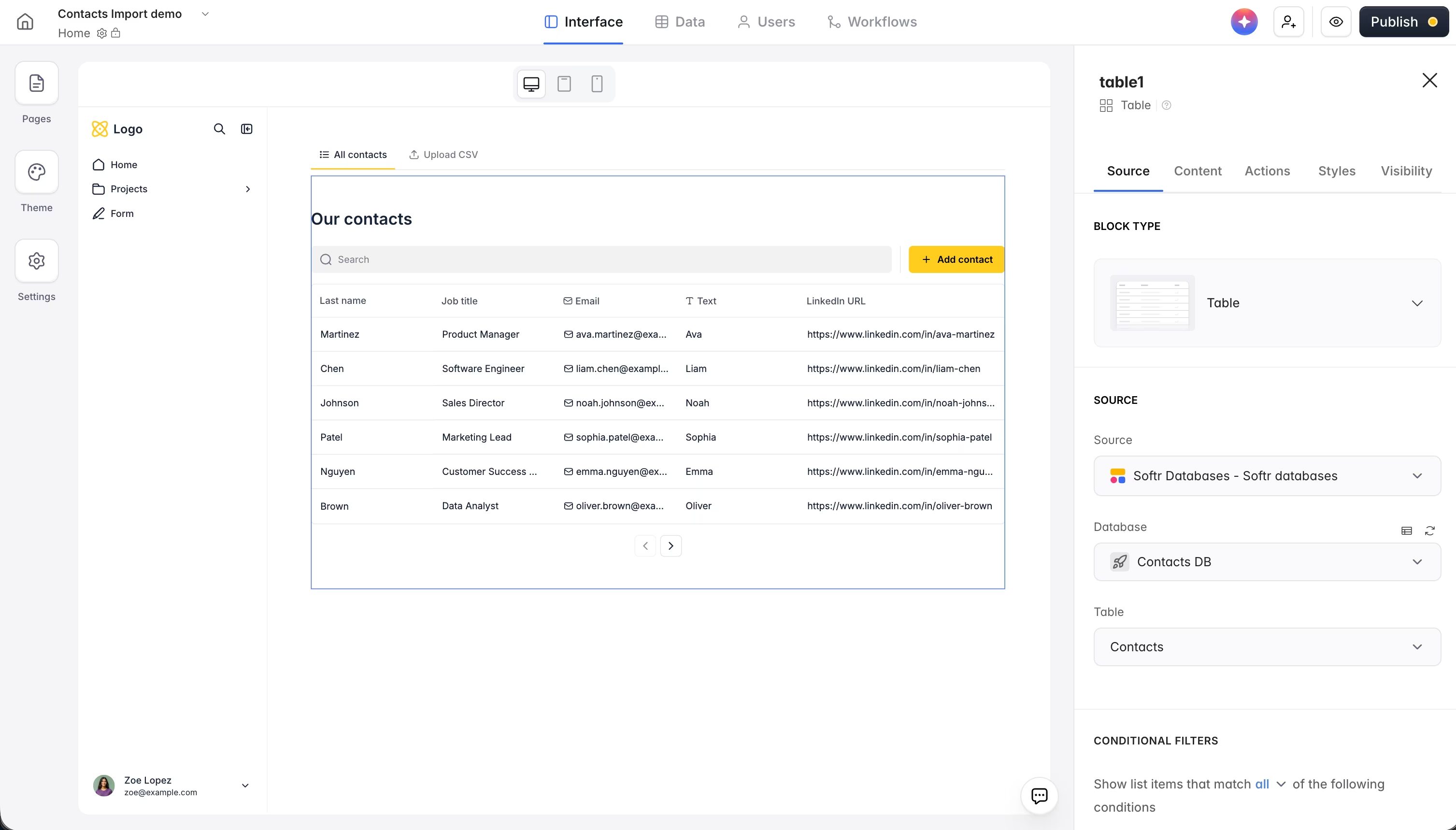
After clicking the “+,” you'll find a sidebar with various blocks and components. In the dynamic tab of the sidebar, click on any of the list blocks.

Step 5: Choose from which Google Sheet file you want to import the data
In the SOURCE tab, click on the drop-down list under “Source.” There, select your connected Google Sheets account. Next, under “Document,” choose the spreadsheet with the data you want to use. Then, under “Sheet,” select the specific sheet within the spreadsheet you selected to import its data.

Step 6: Click “Conditional Filters” in the List settings sidebar
Scroll down the “Source tab” to find and click on the “conditional filters” option. Then click on the “Add condition” button to define your search criteria, so you can filter and display only the data that matches what you need.

Step 7: Test and optimize
Click on the “preview” button to test and ensure the filter(s) is working well.

How to slice data in Google Sheets using the QUERY function
Cost: $0
Time: 1 minute
The QUERY function in Google Sheets is particularly useful when slicing specific subsets of data from a larger dataset based on specified conditions. While the QUERY function has more flexibility than data slicers for handling complex data manipulations, you need a basic understanding of SQL-like syntax.
Below is how you can use the QUERY function to slice data in Google Sheets.
Step 1: Select the cell where you want your filtered data to appear and type the QUERY formula
After selecting the cell where you want the results of the QUERY function to appear, it’s time to use the function to extract the data.
In our example, if you wanted to filter the data to show sales data for the Electronics category in the North region, your QUERY formula would look like this: =QUERY(A:D, "SELECT * WHERE A = 'Electronics' AND B = 'North'"), where:
- A:D refers to the range of columns containing your data
- "SELECT *" selects all columns
- "WHERE A = 'Laptop' AND B = 'North'" specifies the conditions for filtering. You can adjust these conditions based on your needs
The function ensures only laptops in the North region are displayed.

Step 2: Perform advanced functions (optional)
You can also use the QUERY function to aggregate data, such as calculating totals, averages, and counts. For example, to find the total sales amount for "Laptop" in the "North" region, your formula is: =QUERY(A:D, "SELECT SUM(D) WHERE A = 'Laptop' AND B = 'North' LABEL SUM(D) ''")

You can also sort the results using the ORDER BY clause. For example, to sort sales data by date in descending order: =QUERY(A:D, "SELECT * ORDER BY C DESC")

Which method should you use?
Pick the data slicer for quick, one-off filtering on a single sheet. Reach for the QUERY function when you need SQL-like control or aggregations and don't mind the syntax. But once more than one person needs to slice the same data without overwriting each other's views, a Softr app is the better home: filtered list and table views, search, and operational dashboards sit on top of the exact same Google Sheet.

Turn your sliced data into a usable tool
Slicers and formulas are great for answering a quick question inside a spreadsheet. When that data needs to become something your team actually uses every day, put a Softr app on top of it. Connect your Google Sheet, describe the views you need to the AI Co-Builder, and give everyone their own filtered slice without touching the underlying data.
Frequently asked questions
What does it mean to slice data in Google Sheets?
What is the difference between a slicer and a filter in Google Sheets?
When should I use the QUERY function instead of a slicer?
Can multiple people slice the same Google Sheet without affecting each other?
Do I need to move my data out of Google Sheets to build a Softr app?