How to highlight duplicates in Google Sheets

[.blog-callout]

TL;DR

• Select your data range, open Format > Conditional formatting, and choose Custom formula is.
• Use =COUNTIF($A$2:$A$23, $A2)>1 to highlight duplicates in one column, or extend the range to check duplicates across multiple columns.
• Conditional formatting only changes how duplicate cells look. It does not stop new duplicates from being created.
• If duplicate data keeps coming back, the more durable fix is a database with unique fields and validation rules, like Softr Databases. [.blog-callout]

Effective data analysis often involves identifying and reviewing duplicate entries within a dataset. Google Sheets offers a built-in feature that lets you highlight duplicates using conditional formatting, making it easier to spot recurring data points and clean up your spreadsheet before it causes downstream errors.

In this article, we will guide you through the process of highlighting duplicates in Google Sheets using a custom conditional formatting formula, and what to do once your spreadsheet outgrows manual checks like this one.

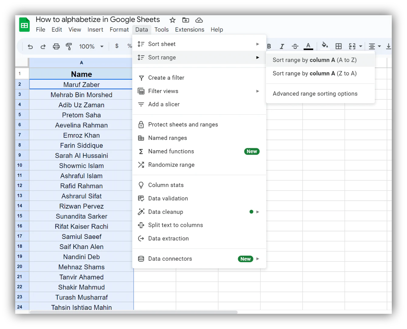
Select the range of cells that you want to highlight duplicates

To select the range of cells you want to check for duplicates, click on one cell and then drag your mouse to select the desired cells.

Open the Conditional format rules panel

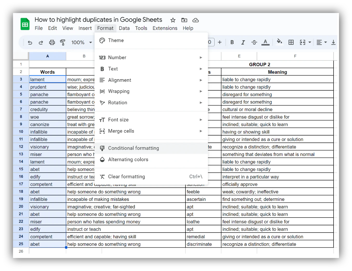
To access the Conditional format rules panel so you can highlight duplicates in your cells, click on the Format menu at the top of the page, then click Conditional formatting.

Format cells based on a custom formula

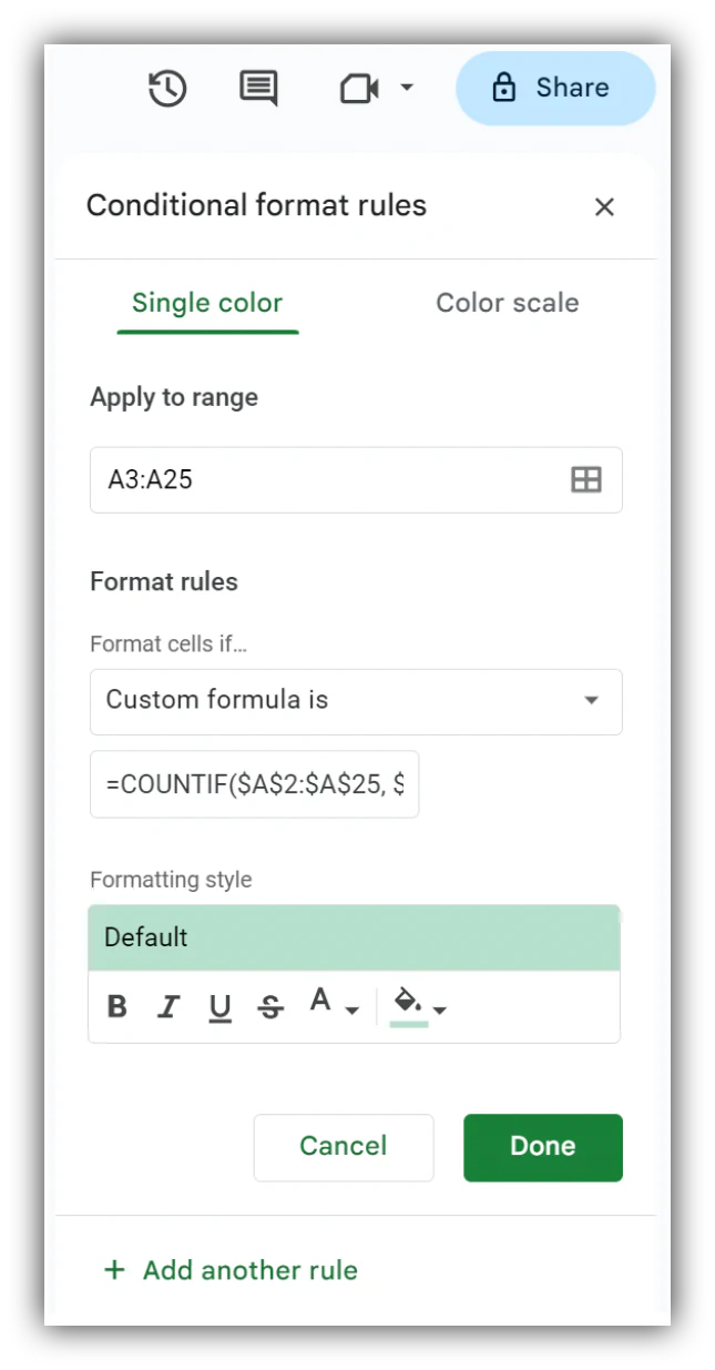
To find duplicates, you need to change the formatting of the cells based on a custom formula. In the Conditional formatting rules panel, specifically in the Format rules section, click on the Format cells if… menu and select Custom formula is.

Add custom formula

Add the following formula to highlight the cells with duplicate content: =COUNTIF($A$2:$A$23, $A2)>1

This formula assumes that the data you want to check for duplicates is in column A and that you want to apply the formatting to the range A2:A23. Modify the formula and range as needed for your own dataset.

Tip: If you want to highlight duplicates across multiple columns too, use the formula =COUNTIF($A$2:$F$25,A2)>1. This checks for duplicates across the range from A2 to F25, so adjust the formula to match your own data range.

Customize formatting style

In the Formatting style section of the Conditional format rules panel, choose how you want to highlight the duplicate cells. In our example, we choose a yellow background to make the duplicates stand out. Once you've finished choosing a formatting style, click Done.

Your duplicates are now highlighted

The duplicate cells in your Google Sheets are now highlighted according to the formatting style you chose, making it much faster to spot and review repeated entries.

When highlighting duplicates isn't enough

Conditional formatting is a quick way to spot duplicates that already exist, but it doesn't stop new ones from being created, and it gets harder to manage as your spreadsheet grows to thousands of rows across multiple tabs. This is usually a sign that a spreadsheet has outgrown its job and it's time for a proper database.

"Primary fields must be as unique as possible. A first name is not a great choice because you might have two people called Jane. Email is a great, unique identifier." - Guillaume Duvernay, Builder at Softr

With Softr Databases, you set a field (like an email address) as a unique identifier, so duplicate records get flagged or rejected automatically at the point of entry instead of after the fact. You can also add a database AI agent to a field to catch inconsistent entries (like "TBD" typed into a date column), or use a Softr Workflow with a search-and-branch step that checks whether a record already exists before creating a new one, which is especially useful for things like lead capture forms where the same contact might submit twice.

Best of all, you don't have to start from scratch. You can import your existing Google Sheet directly into a Softr Database, keep working with the same data, and layer in the validation rules that a spreadsheet can't enforce on its own.