Top Google Sheets formulas that actually work: A cheat sheet

Google Sheets ships with over 500 built-in formulas, but most people only ever need a fraction of them. This guide covers the 100 formulas people actually search for, grouped by category, each with its syntax, a plain-English explanation, and a quick example.

Whether you're running a quick COUNTIF or working out whether XLOOKUP can replace your VLOOKUP and INDEX/MATCH combo, you should be able to find it here.

One thing worth saying up front: if you're reaching for these formulas to run an actual business process, a tracker, a client list, an approval flow, you're often trying to make a spreadsheet behave like an app. That's exactly what Softr is built for, and there's more on when to make that jump at the end.

Most searched formulas

These 20 formulas make up roughly 40% of all the traffic our formula pages get. Start here if you're not sure where to look.

• COUNTIF (Math): Counts how many cells in a range satisfy a single condition, whether that's an exact match, a text string, or a comparison.
• REGEXMATCH (Text): Checks whether a text string contains a pattern described by a regular expression, returning TRUE or FALSE rather than the match itself.
• T.TEST (Statistical): Runs a Student's t-test on two data ranges and returns the p-value indicating whether their means differ significantly.
• SEQUENCE (Math): Generates an array of numbers following a set pattern, filling a grid of the size you specify.
• FORECAST (Statistical): Predicts a y-value for a given x by fitting a linear regression line through existing paired data points.
• MID (Text): Pulls a substring out of a text string starting at a given character position and running for a specified length.
• ROUND (Math): Rounds a number to a specified number of decimal places using standard rounding rules, where anything at or above .5 rounds up.
• IFS (Logical): Tests a series of conditions in order and returns the value tied to the first one that's true, replacing a chain of nested IF statements.
• LINEST (Array): Fits a least-squares line to a set of data points and returns statistics like slope and y-intercept as an array.
• LEFT (Text): Grabs a set number of characters from the start of a text string, useful for trimming codes, prefixes, or truncating labels.
• COUNTIFS (Math): Counts cells that satisfy multiple conditions across one or more ranges simultaneously, extending COUNTIF beyond a single criterion.
• UPPER (Text): Converts every letter in a text string to uppercase, leaving numbers and punctuation untouched.
• GOOGLETRANSLATE (Google): Translates a text string from one language to another directly inside a cell, powered by Google Translate.
• TODAY (Date): Pulls the current date from the system clock and displays it in the sheet's default date format, updating automatically whenever the sheet recalculates.
• ROW (Lookup): Returns the row number of a given cell reference, or of the cell containing the formula itself if no reference is provided.
• IMPORTDATA (Web): Pulls data from a publicly accessible URL, such as a CSV or TSV file, directly into the sheet starting at the cell where the formula sits.
• MROUND (Math): Rounds a number to the nearest multiple of a factor you specify, rather than to a fixed number of decimal places like ROUND.
• REGEXREPLACE (Text): Finds text matching a regular expression pattern and swaps it out for a replacement string, across every match in the cell.
• WEEKDAY (Date): Returns a number representing the day of the week for a given date, useful for scheduling logic or highlighting weekends.
• TEXTJOIN (Text): Concatenates multiple text values or array ranges into one string, inserting a chosen delimiter between each piece.

{{cta-1}}

Math formulas

The everyday counting, rounding, and summing formulas most spreadsheets run on.

COUNTIF

COUNTIF(range, criterion)

Counts how many cells in a range satisfy a single condition, whether that's an exact match, a text string, or a comparison. Criteria support operators like ">" or "<", so you can tally cells above or below a threshold without touching text criteria at all.

=COUNTIF(A1:A10, ">5")

Counts cells in A1:A10 greater than 5.

COUNTIFS

COUNTIFS(criteria_range1, criterion1, [criteria_range2, criterion2, ...])

Counts cells that satisfy multiple conditions across one or more ranges simultaneously, extending COUNTIF beyond a single criterion. You can chain up to 127 range-criterion pairs, mixing comparison operators, wildcards, and cell references across different columns in the same formula.

=COUNTIFS(A1:A10, "apple", B1:B10, ">5")

Counts rows where A is "apple" and B is greater than 5.

COUNTUNIQUE

COUNTUNIQUE(value1, [value2, ...])

Counts how many distinct values appear across one or more ranges or lists, treating duplicates as a single entry. It's a quick way to answer how many different categories exist in a column without building a pivot table or filtering the data first.

=COUNTUNIQUE(A2:A10)

Number of distinct values in A2:A10.

MOD

MOD(dividend, divisor)

Divides one number by another and returns only the remainder, not the quotient. It's the standard way to test divisibility or alternate behavior every nth row, since a MOD result of 0 means the dividend divides evenly into the divisor.

=MOD(10, 3)

Returns 1.

MROUND

MROUND(value, factor)

Rounds a number to the nearest multiple of a factor you specify, rather than to a fixed number of decimal places like ROUND. It's handy for tasks like rounding prices to the nearest nickel or scheduling times to the nearest 15-minute block.

=MROUND(23, 5)

Returns 25.

PI

PI()

Returns the mathematical constant pi, accurate to 14 decimal places, and takes no arguments at all. It's typically nested inside geometry or trigonometry formulas, such as computing a circle's circumference as 2 times PI() times the radius.

=2*PI()*A1

Returns the circumference of a circle with radius in A1.

POWER

POWER(base, exponent)

Raises a base number to a specified exponent, working identically to the ^ operator but as an explicit function call. It's handy for squaring or cubing values inside more complex nested formulas, where the ^ symbol could get visually lost among parentheses.

=POWER(4, 2)

Returns 16.

RAND

RAND()

Generates a random decimal number between 0 (inclusive) and 1 (exclusive), recalculating to a new value each time the sheet updates. Because it takes no arguments and refreshes constantly, it's often combined with ROUND or multiplication to simulate random selections, test data, or shuffling rather than used as a static value.

=RAND()

Returns a random decimal like 0.583921.

RANDBETWEEN

RANDBETWEEN(low, high)

Generates a random integer between two bounds, inclusive of both endpoints, recalculating every time the sheet updates. It's often used for sampling, test data, or shuffling, but the value changes on every edit unless you paste it in as a static number.

=RANDBETWEEN(1, 10)

Returns a random integer from 1 to 10.

ROUND

ROUND(value, [places])

Rounds a number to a specified number of decimal places using standard rounding rules, where anything at or above .5 rounds up. Leaving the places argument out rounds to the nearest whole number instead of a decimal.

=ROUND(3.14159, 2)

Returns 3.14.

ROUNDDOWN

ROUNDDOWN(value, [places])

Truncates a number toward zero to a set number of decimal places, ignoring standard rounding rules entirely. Omitting the places argument rounds to the nearest whole number, and unlike ROUND, it never rounds up no matter how close the decimal portion is to the next increment.

=ROUNDDOWN(3.14159, 2)

Returns 3.14.

ROUNDUP

ROUNDUP(value, [places])

Pushes a number to the next higher value at whatever decimal place you choose, ignoring normal rounding rules entirely. Even a tiny remainder like 3.141 forces a jump to 3.15 with two decimal places, and leaving the places argument off rounds up to the nearest whole number instead.

=ROUNDUP(3.14159, 2)

Returns 3.15.

SEQUENCE

SEQUENCE(rows, columns, start, step)

Generates an array of numbers following a set pattern, filling a grid of the size you specify. You control rows and columns independently, plus the starting value and step size, so setting columns to 1 produces a single vertical list instead of a spread-out grid.

=SEQUENCE(5, 1, 10, 2)

Returns a column of 5 numbers: 10, 12, 14, 16, 18.

SIGN

SIGN(value)

Tells you whether a number is positive, negative, or zero by returning 1, -1, or 0 respectively. It's handy inside larger formulas that need to flip behavior based on a value's direction, such as multiplying a magnitude by SIGN() to preserve whether a change was an increase or decrease.

=SIGN(-10)

Returns -1.

SQRT

SQRT(value)

Calculates the positive square root of a number, returning an error if the input is negative. It's the standard tool for distance, geometry, and statistical formulas like standard deviation, where only the principal positive root is meaningful.

=SQRT(16)

Returns 4.

SUBTOTAL

SUBTOTAL(function_code, range1, [range2, ...])

Aggregates a range using a function you select via a numeric code, such as sum, average, or count, and is commonly used on filtered data. Function codes 1-11 include hidden rows in the calculation, while the equivalent 101-111 codes exclude them, and it automatically ignores other SUBTOTAL formulas nested in its range to avoid double-counting.

=SUBTOTAL(9, A1:A10)

Sums only the visible cells in A1:A10.

SUM

SUM(value1, [value2, ...])

Adds up a series of numbers, cells, or ranges passed in as arguments. It happily mixes individual values with ranges in the same formula and simply ignores any text or blank cells it encounters instead of throwing an error, which makes it forgiving on messy data.

=SUM(A1:A3)

Adds the values in A1, A2, and A3.

Text formulas

Formulas for cleaning, extracting, and reshaping text, including Google's regex functions.

ASC

ASC(text)

Converts full-width characters, common in Japanese text like double-byte katakana or Roman letters, into their half-width equivalents, leaving standard single-byte characters untouched. It's mainly useful for cleaning up text imported from Japanese systems where full-width and half-width characters end up mixed inconsistently.

=ASC("Ａ１")

Returns "A1" in half-width form.

CLEAN

CLEAN(text)

Strips non-printable characters, like line breaks, tabs, and stray control codes, out of a text string while leaving visible characters untouched. It's a common first step when tidying up data pasted or imported from another system, often paired with TRIM to also clear extra spaces.

=CLEAN(A1)

Returns the text in A1 with hidden control characters removed.

CODE

CODE(string)

Returns the numeric Unicode value corresponding to the first character of a text string, ignoring everything after it. It pairs naturally with CHAR, which does the reverse conversion, making the two useful together for encoding tricks or checking whether text starts with a particular character.

=CODE("A")

Returns 65.

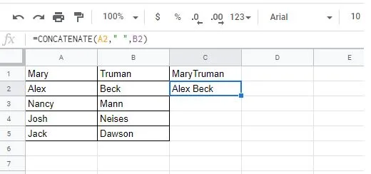
CONCATENATE

CONCATENATE(string1, [string2, ...])

Joins multiple strings, numbers, or cell values into one continuous string, in the order you list them. It accepts up to 30 arguments but has no built-in delimiter, so spaces or punctuation between values must be added manually, unlike TEXTJOIN.

=CONCATENATE(A1, " ", B1)

Combines "Hello" and "World" into "Hello World".

DOLLAR

DOLLAR(number, [number_of_places])

Converts a number into a currency-formatted text string using your spreadsheet's locale symbol. The optional second argument sets how many decimal places to show; leave it out and Sheets defaults to two, rounding the value to fit.

=DOLLAR(1234.567, 2)

Returns "$1,234.57".

EXACT

EXACT(string1, string2)

Compares two strings character by character and confirms whether they match exactly, including capitalization. That case sensitivity is the key detail: a regular equals sign (=) comparison in Sheets ignores case, so EXACT is the one to reach for when "Apple" and "apple" need to be treated as different.

=EXACT("Apple", "apple")

Returns FALSE.

JOIN

JOIN(delimiter, value_or_array1, [value_or_array2, ...])

Combines the elements of one or more ranges or arrays into a single string, separated by a delimiter of your choice. Unlike CONCATENATE, it accepts entire ranges directly, so joining ten cells with a comma takes one argument instead of typing out each cell reference.

=JOIN("-", A1:A3)

Joins the values in A1:A3 with hyphens, e.g. "Red-Green-Blue".

LEFT

LEFT(string, [number_of_characters])

Grabs a set number of characters from the start of a text string, useful for trimming codes, prefixes, or truncating labels. Omitting the character count defaults to just 1 character, and asking for more characters than the string contains simply returns the whole string without an error.

=LEFT("Hello, World!", 5)

Returns "Hello".

LEN

LEN(text)

Counts every character in a text string, including spaces and punctuation, which makes it handy for validating input length or spotting extra whitespace. It works equally well on a literal string or a cell reference, so it's often combined with TRIM to catch accidental double spaces.

=LEN("Hello, world!")

Returns 13.

MID

MID(string, starting_at, extract_length)

Pulls a substring out of a text string starting at a given character position and running for a specified length. Position counting starts at 1, and if the string is shorter than expected it simply returns whatever characters remain rather than erroring.

=MID("Hello, World!", 8, 5)

Returns "World".

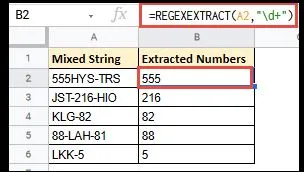
REGEXEXTRACT

REGEXEXTRACT(text, regular_expression)

Searches a text string for a regular expression pattern and pulls out the first matching substring, returning an empty string if nothing matches. It's often used to lift structured data like email addresses or codes out of messier free-text cells.

=REGEXEXTRACT(A1, "[A-Za-z0-9._%+-]+@[A-Za-z0-9.-]+\.[A-Za-z]{2,4}")

Extracts the email address found in A1.

REGEXMATCH

REGEXMATCH(text, regular_expression)

Checks whether a text string contains a pattern described by a regular expression, returning TRUE or FALSE rather than the match itself. Matching is case-sensitive by default, but prefixing the pattern with (?i) makes it case-insensitive.

=REGEXMATCH("Hello World", "World")

Returns TRUE.

REGEXREPLACE

REGEXREPLACE(text, regular_expression, replacement)

Finds text matching a regular expression pattern and swaps it out for a replacement string, across every match in the cell. Both the pattern and the replacement can be cell references instead of hardcoded strings, which makes it easy to strip out characters like vowels or reformat codes in bulk.

=REGEXREPLACE("Hello, world!", "[aeiou]", "")

Returns "Hll, wrld!".

REPLACE

REPLACE(text, position, length, new_text)

Swaps out a specific stretch of a text string, defined by starting position and character length, with new text of your choosing. Unlike SUBSTITUTE, which matches text by content, REPLACE matches by position, so it's the better pick when you know exactly where in the string the change needs to happen.

=REPLACE("Hello, world!", 8, 5, "everyone")

Returns "Hello, everyone!".

RIGHT

RIGHT(string, [number_of_characters])

Pulls a set number of characters from the end of a text string, useful for grabbing suffixes like file extensions or the last few digits of an ID. Leaving the character count out defaults to just one character, and it pairs naturally with LEN when you need everything except the first few characters.

=RIGHT("Hello, World!", 5)

Returns "rld!".

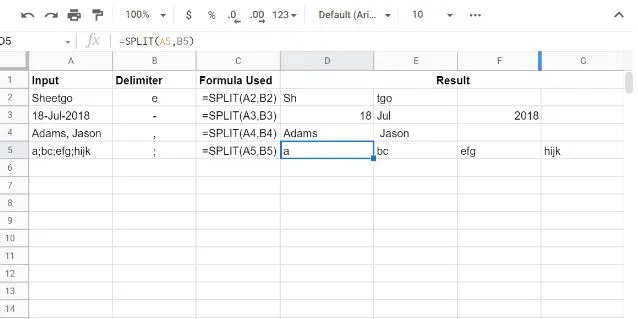
SPLIT

SPLIT(text, delimiter, [split_by_each], [remove_empty_text])

Breaks a text string into separate cells across a row, using whatever delimiter character or string you choose. Setting split_by_each to TRUE treats every character in the delimiter as its own separate split point instead of matching the delimiter as one unit, and remove_empty_text drops blank fragments from the result.

=SPLIT("apple,banana,orange", ",")

Spills "apple", "banana", "orange" into adjacent cells.

SUBSTITUTE

SUBSTITUTE(text_to_search, search_for, replace_with, [occurrence_number])

Finds a piece of text within a string and swaps it for something else, replacing every match by default. Adding the optional occurrence_number argument targets just one specific instance instead of all of them, though note the search itself is case-sensitive.

=SUBSTITUTE("Hello world world", "world", "universe", 2)

Returns "Hello world universe".

TEXTJOIN

TEXTJOIN(delimiter, ignore_empty, text1, [text2], …)

Concatenates multiple text values or array ranges into one string, inserting a chosen delimiter between each piece. The ignore_empty argument, when set to TRUE, skips blank cells so you don't end up with stray delimiters where data is missing.

=TEXTJOIN(", ", TRUE, "Apple", "Banana", "Orange")

Returns "Apple, Banana, Orange".

UPPER

UPPER(text)

Converts every letter in a text string to uppercase, leaving numbers and punctuation untouched. It only affects lowercase letters, so any characters already capitalized in the original text stay exactly as they were.

=UPPER("hello world")

Returns "HELLO WORLD".

VALUE

VALUE(text)

Converts text that looks like a number, date, or time into an actual numeric value Sheets can calculate with, which matters when data imported from elsewhere lands as text. Feeding it a string that can't be parsed as a number throws a #VALUE! error rather than silently returning zero.

=VALUE("123")

Returns 123 as a number.

[.blog-callout] If you regularly run CLEAN, TRIM, SPLIT, and REGEXREPLACE just to keep data usable, that is usually a sign the spreadsheet is doing a database's job. A real database keeps data clean at entry with field types, dropdowns, and validation, so you are not repairing it with formulas afterward. Softr databases give you one to build on directly, and Softr can also sit on top of the Google Sheet or Excel file you already have. [.blog-callout]

Statistical formulas

Formulas for averages, distributions, forecasting, and testing whether a result is significant.

AVERAGE.WEIGHTED

AVERAGE.WEIGHTED(values, weights, [additional values], [additional weights])

Calculates an average where each value counts more or less depending on an assigned weight, rather than treating every entry equally. It multiplies each value by its corresponding weight, sums those products, then divides by the total of the weights, which is exactly how a grade weighted by assignment importance gets computed.

=AVERAGE.WEIGHTED(A1:A5, B1:B5)

Returns the weighted average of A1:A5 using weights in B1:B5.

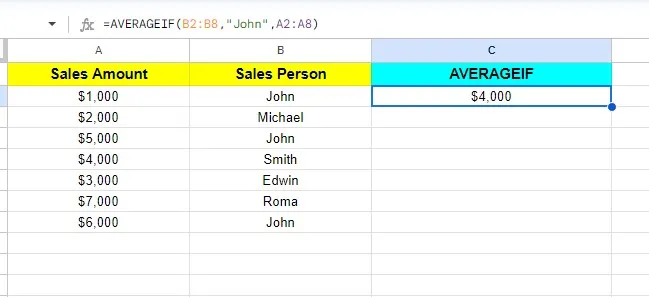
AVERAGEIF

AVERAGEIF(criteria_range, criterion, [average_range])

Averages the cells in a range that satisfy a single condition, checking one column for a criterion and pulling matching values from another. Omitting the average_range makes it average the criteria_range itself, and blank or logical cells that match the criterion are skipped rather than counted as zero.

=AVERAGEIF(B1:B10, "John", A1:A10)

Average of sales in A1:A10 where B1:B10 equals "John".

CHISQ.TEST

CHISQ.TEST(observed_range, expected_range)

Runs a chi-squared test comparing a range of observed values against a range of expected values, returning the probability that any difference between them is due to chance. Both ranges must share the same dimensions, and it's the modern replacement for the older CHITEST function, which Sheets keeps for backward compatibility.

=CHISQ.TEST(A2:A10, B2:B10)

P-value from the chi-squared test.

CONFIDENCE

CONFIDENCE(alpha, standard_deviation, pop_size)

Calculates the margin of error for a population mean from a significance level (alpha), standard deviation, and sample size; add and subtract that margin from the sample mean to build a confidence interval. Common alpha values are 0.05 for 95% confidence and 0.01 for 99%, and the result assumes a normally distributed population or a sample large enough for the Central Limit Theorem to apply.

=CONFIDENCE(0.05, 2.5, 50)

Margin of error at 95% confidence for a sample of 50.

CORREL

CORREL(data_y, data_x)

Measures how closely two variables move together in a straight-line relationship, returning a value from -1 (perfect negative) to 1 (perfect positive). It runs the same underlying calculation as PEARSON, so choosing between them mostly comes down to habit or formula readability.

=CORREL(A2:A10, B2:B10)

Correlation coefficient between the two ranges.

COUNTA

COUNTA(value1, [value2, ...])

Counts every non-empty cell in a range, regardless of whether it holds text, numbers, TRUE/FALSE values, or even an error. That makes it broader than COUNT, which only tallies numeric cells, so COUNTA is the better pick when you just need to know how many rows have been filled in.

=COUNTA(A2:A100)

Returns the count of non-blank cells in A2:A100.

FORECAST

FORECAST(x, data_y, data_x)

Predicts a y-value for a given x by fitting a linear regression line through existing paired data points. It's commonly used to project future figures, like sales for an upcoming year, from historical x-y pairs such as year and revenue.

=FORECAST(A1, B2:B100, A2:A100)

Predicts the y-value for the x in A1 based on historical data in A2:A100 and B2:B100.

FORECAST.LINEAR

FORECAST.LINEAR(x, data_y, data_x)

Predicts a y-value for a given x by fitting a straight line through existing data points using linear regression. It's the modern, clearer-named equivalent of the older FORECAST function, useful for projecting sales or metrics forward when the underlying trend looks roughly linear rather than exponential.

=FORECAST.LINEAR(10, B1:B5, A1:A5)

Predicts the y-value at x=10 based on the trend in A1:A5 and B1:B5.

LARGE

LARGE(data, n)

Pulls the nth largest value out of a range, so setting n to 1 returns the top value, 2 the runner-up, and so on. It's a fast way to rank or spot outliers without sorting the whole dataset, such as pulling the top three sales figures for a report.

=LARGE(A1:A10, 2)

Returns the second-largest value in A1:A10.

MAXIFS

MAXIFS(range, criteria_range1, criterion1, [criteria_range2, criterion2], …)

Finds the largest value in a range after filtering by one or more matching conditions across other ranges. Every criteria_range and criterion pair must line up in size with the main range, and it returns blank if nothing meets all the conditions at once.

=MAXIFS(C:C, A:A, "Product A", B:B, "North")

Returns the highest sales amount for Product A in the North region.

MINIFS

MINIFS(range, criteria_range1, criterion1, [criteria_range2, criterion2], …)

Finds the smallest value in a range, but only considers cells that satisfy one or more corresponding criteria applied to other ranges. Up to 127 criteria pairs can be combined, so it works like MIN with AND logic layered on top, the same way MAXIFS and SUMIFS extend their base functions.

=MINIFS(A1:A10, B1:B10, ">10", C1:C10, "<>0")

Smallest value in A1:A10 where B is over 10 and C isn't 0.

MODE

MODE(value1, [value2, ...])

Finds the value that occurs most often across one or more ranges of numbers, useful for spotting the most common entry in a dataset. If several values tie for the highest frequency it returns the smallest of them, and it errors out entirely if no value repeats at all.

=MODE(A2:A6)

Returns the most frequently occurring number in A2:A6.

NORMDIST

NORMDIST(x, mean, standard_deviation, cumulative)

Calculates probability values for a normal distribution given a value, mean, and standard deviation. Setting the cumulative argument to TRUE returns the probability of a value falling at or below that point, while FALSE returns the density at that exact point, useful for quality control checks and statistical modeling.

=NORMDIST(80, 75, 5, TRUE)

Cumulative probability of scoring 80 or below in that distribution.

PEARSON

PEARSON(data_y, data_x)

Measures the strength and direction of the linear relationship between two data sets, returning a coefficient between -1 and 1. It's mathematically identical to CORREL, so the two are used interchangeably, but both require the input ranges to be the same length or they return an error.

=PEARSON(A2:A10, B2:B10)

Correlation coefficient between the two ranges.

PROB

PROB(data, probabilities, low_limit, [high_limit])

Calculates the probability that a value falls within a given range, based on a matching set of values and their assigned probabilities. It works by summing the probabilities tied to every value between low_limit and high_limit, so the probabilities argument should already add up to 1 for the result to be meaningful.

=PROB(A2:A10, B2:B10, 0, 5)

Returns the summed probability of values between 0 and 5.

QUARTILE

QUARTILE(data, quartile_number)

Returns the value at a specified quartile boundary within a dataset, splitting it into quarters. The quartile_number argument controls which cut point comes back: 0 for the minimum, 1 for the 25th percentile, 2 for the median, 3 for the 75th percentile, and 4 for the maximum.

=QUARTILE(A1:A10, 2)

Returns the median (second quartile) of A1:A10.

RANK

RANK(value, data, [is_ascending])

Returns a value's position within a dataset, from largest to smallest by default. Setting the optional is_ascending argument to TRUE flips the order to smallest-to-largest, and tied values share a rank while the next rank down gets skipped entirely.

=RANK(7, A2:A6)

Returns 7's rank within A2:A6 (2nd largest, descending order).

STDEV

STDEV(value1, [value2, ...])

Measures how spread out a set of values is around their average, calculated from a sample rather than the full population. It accepts up to 255 values or ranges at once, and feeding it a single value or single-cell range returns 0 since there's no variation to measure.

=STDEV(A1:A5)

Returns the sample standard deviation of A1:A5.

T.TEST

T.TEST(range1, range2, tails, type)

Runs a Student's t-test on two data ranges and returns the p-value indicating whether their means differ significantly. Two optional arguments control the test: tails (1 or 2, defaulting to a two-tailed test) and type, where 1 assumes paired samples and 2 assumes independent samples with equal variance.

=T.TEST(A2:A10, B2:B10, 2, 1)

P-value for a two-tailed paired t-test comparing A2:A10 and B2:B10.

[.blog-callout] Formulas like FORECAST, RANK, and the AVERAGEIF family often power a shared reporting sheet. The moment more than a couple of people rely on it, you hit the spreadsheet's real limits: no per-person permissions, and one wrong edit breaks everyone's numbers. Softr turns that data into a proper reporting app with controlled access, built on Softr's own database or on the spreadsheet you already use. [.blog-callout]

Logical formulas

The conditional building blocks (IF, AND, IFS) that most other formulas get wrapped in.

AND

AND(logical_expression1, [logical_expression2, ...])

Evaluates a set of logical conditions and returns TRUE only if every single one of them is true, otherwise FALSE. It's typically paired with other functions like ISBLANK inside a larger formula to check that several requirements are all met at once, up to 255 conditions.

=AND(ISBLANK(A1)=FALSE, ISBLANK(B1)=FALSE)

Returns TRUE if both A1 and B1 contain values.

IFERROR

IFERROR(value, [value_if_error])

Evaluates a formula and returns its result unless that formula produces an error, in which case it returns a fallback value you specify instead. It's the standard way to replace errors like #DIV/0! with a blank, zero, or custom message, without testing for the error condition separately first.

=IFERROR(A1/B1, "Cannot divide by zero")

Shows the division result, or the message if B1 is 0.

IFNA

IFNA(value, value_if_na)

Checks whether a formula's result is specifically the #N/A error, returning a fallback value only in that case while letting any other error type pass through unchanged. It's narrower than IFERROR, useful when you want failed lookups handled differently from other kinds of errors.

=IFNA(VLOOKUP(A1, B:C, 2, FALSE), "Not found")

Shows "Not found" if the lookup returns #N/A.

IFS

IFS(condition1, value1, [condition2, value2], …)

Tests a series of conditions in order and returns the value tied to the first one that's true, replacing a chain of nested IF statements. If none of the conditions evaluate to true, it returns an error, so it's worth including a final catch-all condition to avoid that.

=IFS(A1>=90, "A", A1>=80, "B", A1>=70, "C", A1<70, "F")

Returns a letter grade based on the score in A1.

LET

LET(name1, value_expression1, [name2, …], [value_expression2, …], formula_expression )

Defines named variables inside a single formula and then uses them in a final expression, avoiding repeated subformulas. Each value expression is calculated only once even if referenced multiple times downstream, which keeps complex formulas both readable and efficient.

=LET(a, 5, b, 7, c, a + b, c * 2)

Returns 24.

NOT

NOT(logical_expression)

Flips a logical value to its opposite, turning TRUE into FALSE and FALSE into TRUE. It's most useful nested inside conditions like IF or AND to reverse a test's outcome without rewriting the underlying logic, such as checking that a cell is not blank.

=NOT(ISBLANK(A1))

Returns TRUE if A1 is not blank.

TRUE

TRUE()

Returns the Boolean value TRUE without needing any arguments, acting as an explicit function form of typing the word TRUE directly into a formula. It's most useful inside logical tests or as a default placeholder in IF statements, since a function call is less likely to be misread than a bare keyword.

=IF(TRUE(), "Yes", "No")

Returns "Yes".

Date formulas

Formulas for working with dates, weekdays, and working-day calculations.

EDATE

EDATE(start_date, months)

Shifts a date forward or backward by a whole number of months, automatically handling month-end and year-boundary rollovers that manual date math gets wrong. A negative months value moves the date backward instead, which makes it useful for calculating renewal dates or lookback windows.

=EDATE(A1, 6)

Returns the date 6 months after the date in A1.

NETWORKDAYS.INTL

NETWORKDAYS.INTL(start_date, end_date, [weekend], [holidays])

Counts the working days between two dates while letting you define exactly which days count as the weekend, rather than assuming a fixed Saturday-Sunday schedule. An optional holidays list excludes additional non-working dates, making it more flexible than the plain NETWORKDAYS function for teams on non-standard schedules.

=NETWORKDAYS.INTL(A1, B1, 11)

Working days between A1 and B1, treating only Sunday as a weekend.

TODAY

TODAY()

Pulls the current date from the system clock and displays it in the sheet's default date format, updating automatically whenever the sheet recalculates. It takes no arguments at all, so typing anything between the parentheses will throw an error.

=TODAY()

Returns the current date, e.g. 07/21/2026.

WEEKDAY

WEEKDAY(date, [type])

Returns a number representing the day of the week for a given date, useful for scheduling logic or highlighting weekends. The optional type argument changes the numbering scheme: type 1 (default) runs Sunday=0 through Saturday=6, type 2 runs Monday=1 through Sunday=7, and type 3 returns the day name as text.

=WEEKDAY("2026-07-21", 2)

Returns 2 (Tuesday, Monday-start numbering).

YEAR

YEAR(date)

Pulls just the four-digit year out of a date value, whether that date comes from a cell reference or a quoted date string. It's a simple building block for grouping records by year or comparing dates across different reporting periods.

=YEAR(A1)

Returns the year of the date in A1, e.g. 2023.

Array formulas

Formulas that operate on a whole range at once instead of one cell at a time.

FREQUENCY

FREQUENCY(data, classes)

Groups a column of data into bins you define and counts how many values fall into each one, returning the counts as an array. It's the go-to for building a histogram, like tallying how many test scores land in each 50-point range without manually filtering the data.

=FREQUENCY(A1:A20, B1:B4)

Returns counts of A1:A20 values falling into each class defined in B1:B4.

GROWTH

GROWTH(known_data_y, [known_data_x], [new_data_x], [b])

Fits an exponential curve to known data and projects future values along that curve, which suits metrics that compound rather than grow linearly, like traffic doubling month over month. Give it new x-values as the third argument and it returns predicted y-values for those points instead of just describing the existing trend.

=GROWTH(B2:B6, A2:A6, A7:A8)

Predicts values for the two new periods in A7:A8 based on the exponential trend in A2:B6.

LINEST

LINEST(known_data_y, [known_data_x], [calculate_b], [verbose])

Fits a least-squares line to a set of data points and returns statistics like slope and y-intercept as an array. Setting the third and fourth arguments to TRUE returns the full verbose statistics output rather than just the slope, useful for deeper regression analysis beyond a single forecast.

=LINEST(B2:B6, A2:A6, TRUE, TRUE)

Returns the slope, intercept, and regression stats for the data in A2:A6 and B2:B6.

SUMPRODUCT

SUMPRODUCT(array1, [array2, ...])

Multiplies corresponding elements across one or more equally sized arrays, then adds all those products into a single number. Beyond straightforward math, it's often used as a workaround for conditional counting and weighted averages, since it can multiply logical TRUE/FALSE arrays without an array-entered formula.

=SUMPRODUCT(A1:A5, B1:B5)

Sum of A1B1 + A2B2 + ... + A5*B5.

TREND

TREND(known_data_y, [known_data_x], [new_data_x], [b])

Fits a least-squares straight line to known x and y data and can extend that line to predict y-values for new x inputs, returning an array rather than a single number. Skip the known_data_x argument and it assumes x-values of 1, 2, 3... automatically, and setting the optional b argument to TRUE forces the line through the origin.

=TREND(A1:A5, B1:B5, C1:C3)

Predicts y-values for the new x-values in C1:C3.

Lookup formulas

Formulas for finding a value in one place and pulling data from another (VLOOKUP and its relatives).

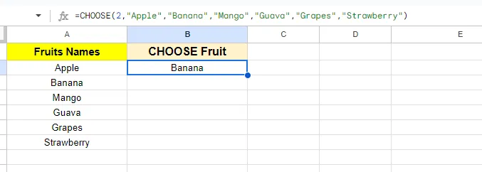
CHOOSE

CHOOSE(index, choice1, [choice2, ...])

Picks and returns one value from a list of choices based on a numeric index position. The index must be a whole number between 1 and 254, and if it falls outside that range or has no matching choice, the formula returns an error rather than the nearest valid option.

=CHOOSE(2, A1, A2, A3, A4)

Returns the value stored in A2.

COLUMN

COLUMN([cell_reference])

Returns the column number for a given cell reference, counting A as 1, B as 2, and so on. Leave the argument out and it returns the column number of the cell holding the formula itself, which is handy for building references that shift automatically as you copy across columns.

=COLUMN(C4)

Returns 3.

GETPIVOTDATA

GETPIVOTDATA(value_name, any_pivot_table_cell, [original_column, ...], [pivot_item, ...]

Pulls a single aggregated number out of a pivot table by matching the row and column labels you specify, rather than by raw cell position. That makes it more resilient than a plain reference, since it keeps pointing at the right figure even after the pivot table is resorted or resized.

=GETPIVOTDATA("Sum of Sales", A3, "Region", "East")

Returns the summed sales value for the East region.

INDEX

INDEX(reference, [row], [column])

Returns the value at a specific row and column position within a given range, working like a coordinate lookup rather than a search. Leave out the row or column argument and it returns the entire corresponding row or column instead, which is why it's so often paired with MATCH to build flexible two-way lookups.

=INDEX(A1:B10, 3, 2)

Returns the value in the 3rd row, 2nd column of A1:B10.

INDIRECT

INDIRECT(cell_reference_as_string, [is_A1_notation])

Turns a text string into an actual cell reference, letting a formula point to a different cell dynamically based on another cell's value. It supports both A1 and R1C1 notation via its second argument, and is often used to build references that shift with a dropdown, though it can slow down large sheets since it recalculates constantly.

=INDIRECT("A1")

Returns the value stored in cell A1.

LOOKUP

LOOKUP(search_key, search_range|search_result_array, [result_range])

Searches one row or column for a key and returns the value from the matching position in a separate result range. It requires the search range to be sorted in ascending order to work reliably, which is why VLOOKUP or INDEX/MATCH are usually the safer choice for unsorted data.

=LOOKUP(10, A2:A10, B2:B10)

Returns the B-column value matching the largest A-value at or below 10.

ROW

ROW([cell_reference])

Returns the row number of a given cell reference, or of the cell containing the formula itself if no reference is provided. This makes it handy for building dynamic references, like generating incrementing values as a formula is copied down a column.

=ROW(A5)

Returns 5.

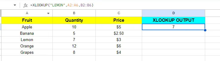
XLOOKUP

XLOOKUP(search_key, lookup_range, result_range, missing_value, [match_mode], [search_mode])

Searches a range for a matching value and returns the corresponding result from a separate range, without requiring the lookup and result columns to sit next to each other like VLOOKUP demands. It also lets you set a fallback for no match, plus optional match modes (exact, next larger/smaller, wildcard) and search direction for large or unordered data.

=XLOOKUP(A2, B:B, C:C, "Not found")

Matching value from column C, or "Not found".

[.blog-callout] If you are chaining VLOOKUP or INDEX/MATCH across multiple tabs to connect records, that is exactly what a database does natively, without the broken references every time someone inserts a row. Softr databases keep the same rows and columns you are used to, but with real relationships between tables instead of lookup formulas holding everything together. [.blog-callout]

Parser formulas

Formulas that convert a value from one format to another, like a number into a date.

CONVERT

CONVERT(value, start_unit, end_unit)

Translates a numeric value from one unit of measurement into another, covering length, weight, time, volume, temperature, and more. It's built for switching between measurement systems, like turning inches into centimeters or pounds into kilograms, without writing a manual conversion formula.

=CONVERT(1, "in", "cm")

Converts 1 inch to centimeters (2.54).

TO_DATE

TO_DATE(value)

Converts a numeric value or date-time serial into a proper date format, stripping away any time component. It's useful when a cell holds a combined date and time value but downstream formulas, sorting, or filtering only need the date portion.

=TO_DATE(A1)

Converts the value in A1 to a date.

TO_PERCENT

TO_PERCENT(value)

Reformats a decimal or fraction so it displays as a percentage, without changing the underlying numeric value. It's a formatting shortcut more than a calculation: 0.75 becomes 75%, making reports and charts read more naturally than raw decimals would.

=TO_PERCENT(0.75)

Displays 0.75 as 75%.

TO_TEXT

TO_TEXT(value)

Converts a number, date, or boolean into its plain text representation, stripping away any numeric or date formatting so the result behaves like a string in later formulas. Useful before concatenating values, since mixing raw numbers with text elsewhere can trigger unexpected type coercion or formatting mismatches.

=TO_TEXT(42)

Returns the text string "42".

Info formulas

Formulas that check what's actually in a cell: blank, error, text, or number.

CELL

CELL(info_type, reference)

Reports metadata about a specified cell, such as its address, formatting code, or content type, depending on the info_type keyword you pass in. Different keywords unlock different details: "format" returns something like "0.00" while "address" returns the cell's reference string.

=CELL("address", A1)

Returns "$A$1".

ISBLANK

ISBLANK(value)

Tests whether a cell has any content, returning TRUE if it's empty and FALSE if it holds anything, including a space or a formula that outputs an empty string. It's most useful nested inside an IF statement to skip calculations or flag missing entries before they cause errors elsewhere.

=ISBLANK(A1)

Returns TRUE if A1 is empty, FALSE otherwise.

ISDATE

ISDATE(value)

Checks whether a given value is a recognized date and returns TRUE or FALSE accordingly. It's useful for validating imported data before running date-based calculations, since a value that merely looks like a date but is stored as plain text will return FALSE.

=ISDATE(A1)

Returns TRUE if A1 contains a valid date.

ISNUMBER

ISNUMBER(value)

Checks whether a given value is numeric, returning TRUE or FALSE accordingly. It's especially useful for cleaning up mixed columns where text and numbers are jumbled together, letting you filter or flag rows before running calculations that would otherwise error out on text.

=ISNUMBER(A1)

Returns TRUE if A1 contains a number, FALSE otherwise.

Google formulas

Formulas unique to Google Sheets, like translation and stock data.

GOOGLETRANSLATE

GOOGLETRANSLATE(text, [source_language], [target_language])

Translates a text string from one language to another directly inside a cell, powered by Google Translate. The source language argument is optional and defaults to "auto," letting the function detect the input language on its own before translating to the target.

=GOOGLETRANSLATE("Hello world", "en", "es")

Returns "Hola Mundo".

IMAGE

IMAGE(url, [mode], [height], [width])

Embeds a picture from a web URL directly inside a cell, rather than floating it over the sheet like an inserted image object. The mode argument controls sizing: 1 fits the image within the given dimensions while keeping its aspect ratio, and 2 stretches or squashes it to fill the height and width exactly.

=IMAGE("https://example.com/logo.png", 1, 50, 50)

Displays the logo sized to fit within a 50x50 box.

SPARKLINE

SPARKLINE(data, [options])

Draws a compact line, bar, column, or win/loss chart inside a single cell, built from a range of data you supply. The optional options argument, passed as a two-column array, lets you set chart type, colors, and axis min/max without ever opening the full chart editor.

=SPARKLINE(A1:A10, {"charttype","column"})

Shows a small column chart of A1:A10 inside the cell.

Web formulas

Formulas that pull external data into a sheet.

ENCODEURL

ENCODEURL(text)

Escapes a text string into a URL-safe format, replacing spaces, commas, and other special characters with their percent-encoded equivalents. It's essential when building a URL dynamically from cell values, such as constructing a search or query link where the input might contain spaces or punctuation.

=ENCODEURL("Hello, World!")

Returns "Hello%2C%20World%21".

IMPORTDATA

IMPORTDATA(url)

Pulls data from a publicly accessible URL, such as a CSV or TSV file, directly into the sheet starting at the cell where the formula sits. Imported data refreshes roughly every hour and overwrites whatever was already in the destination cells, so it won't work with URLs that require login.

=IMPORTDATA("https://example.com/data.csv")

Imports the CSV data from that URL into the sheet.

IMPORTXML

IMPORTXML(url, xpath_query)

Fetches structured data from a webpage or feed by running an XPath query against its XML or HTML source, returning an array of matching values. It fails on pages that require login or rely heavily on JavaScript rendering, and Google may throttle or block repeated high-volume requests to the same site.

=IMPORTXML("https://example.com", "//h1")

Returns the text of the page's first h1 heading.

[.blog-callout] IMPORTRANGE and IMPORTDATA exist to pull data from one place into another, usually the first sign you have outgrown a single sheet. Rather than stitching sheets together, Softr can build a real app on top of the Google Sheet or Excel file you already use, so the data stays put but gains an interface, logins, and permissions. When you need to scale further, Softr's own database is faster and holds far more than a spreadsheet can. [.blog-callout]

Operator formulas

The named function equivalents of +, -, =, and other operators.

EQ

EQ(value1, value2)

Compares two values and returns TRUE if they match exactly, FALSE otherwise, doing the same job as typing an = sign between two cells. It exists mainly for compatibility with other spreadsheet systems and for cases needing an explicit function rather than an infix operator, such as inside ARRAYFORMULA.

=EQ(A1, B1)

Returns TRUE if A1 and B1 hold the same value.

ISBETWEEN

ISBETWEEN(value_to_compare, lower_value, upper_value, lower_value_is_inclusive, upper_value_is_inclusive)

Checks whether a number falls within a lower and upper boundary, letting you set each boundary as inclusive or exclusive independently instead of assuming one fixed rule. That flexibility makes it handy for range validation where "between 5 and 10" needs to mean something different depending on context, like grading bands or date filters.

=ISBETWEEN(A1, 5, 10, TRUE, TRUE)

TRUE if A1 holds 7.

UMINUS

UMINUS(value)

Reverses the sign of a number, turning a positive value negative and a negative value positive, functionally identical to putting a minus sign in front of it. It rarely gets typed by hand but is the underlying operator behind shorthand formulas like =-A1.

=UMINUS(A1)

Returns -5 if A1 contains 5.

Financial formulas

Loan, interest, and depreciation formulas.

NPV

NPV(discount, cashflow1, [cashflow2, ...])

Discounts a series of future cash flows back to their present value using a fixed discount rate, a standard check for whether an investment or project is worth pursuing. The cash flows are assumed to land at regular, equal intervals, so unevenly timed payments call for XNPV instead.

=NPV(0.1, -10000, 3000, 4200, 6800)

Returns the net present value of the cash flow series at a 10% discount rate.

PMT

PMT(rate, number_of_periods, present_value, [future_value], [end_or_beginning])

Calculates the fixed periodic payment needed to pay off a loan or fund an investment at a constant interest rate over a set number of periods. The optional end_or_beginning argument controls whether payments land at the end (0, the default) or start (1) of each period, which slightly changes the result for annuities-due.

=PMT(0.05/12, 60, 20000)

Monthly payment on a $20,000 loan at 5% over 60 months.

When a spreadsheet stops being enough

Formulas like VLOOKUP, QUERY, and IMPORTRANGE exist because people are trying to make Google Sheets behave like a database: filtering, joining, and pulling data from one place into another. That works, until the sheet has multiple editors, the formulas start breaking when someone inserts a row, or you need permissions so not everyone can see or edit everything.

At that point the fix usually isn't a better formula, it's giving the data a real home and a real interface. Softr is built for exactly this: describe the tool you need (a client portal, an internal tracker, a CRM) and it builds a secure, working web app, with logins, roles, and permissions handled for you. You can build on Softr's own database, which is faster and scales well past spreadsheet limits, or connect the Google Sheet, Excel file, or Airtable base you already use as the data source.

You keep the part of a spreadsheet you liked, a familiar grid you can edit, without the parts you didn't: broken formulas, no permissions, and one shared tab anyone can wreck.

{{cta-2}}