How to search in Google Sheets

[.blog-callout]

TL;DR

• The fastest way to search a single sheet is the keyboard shortcut (Ctrl + F or Cmd + F). For multi-tab searches, use Find and Replace with the All sheets option.
• For more control, use filter views, conditional formatting, or lookup functions like VLOOKUP, HLOOKUP, INDEX/MATCH, and QUERY.
• These methods work well for one person, but spreadsheet filters are global, so they collide as soon as a team shares the file.
• When two or more people rely on a sheet every week to find records, it's usually time to build a real app with search, filters, and permissions on top of your data using Softr. [.blog-callout]

Google Sheets has a search feature that helps you quickly find the exact information you need, which is handy when you're sorting through lots of data. Whether you're correcting a typo across hundreds of rows or pulling a single price out of a product table, the right method saves you from scrolling forever.

This article breaks down how to search in Google Sheets using nine different methods. For each one, we cover the use case, how long it takes, the cost, and how to use it. We'll also look at what happens when a spreadsheet outgrows search, and how a tool like Softr lets you build a proper internal tool with real search and filters on top of the same data. Here's a quick rundown of each method.

1. Find and Replace: quickly search for specific data in your spreadsheet and replace it with new information.
2. Softr search interface: build a searchable app on top of your sheet, handling multiple criteria, conditions, and patterns that go beyond what Google Sheets functions can do.
3. Keyboard shortcuts: one of the quickest ways to search a single sheet.
4. Conditional formatting: visually highlight and format cells based on specific conditions.
5. Filter views: create custom filtered versions of your data without affecting the view for others.
6. VLOOKUP function: look up certain data in your spreadsheet by searching the first column.
7. HLOOKUP function: search for a value in a row and retrieve a corresponding value from another row.
8. INDEX and MATCH functions: combine these to search by various criteria and retrieve data from different rows and columns.
9. QUERY function: perform SQL-like queries on your data.

How to search in Google Sheets using Find and Replace

Cost: $0

Time: 1 minute

The "Find and Replace" feature in Google Sheets allows you to quickly search for specific data in your spreadsheet and replace it with new information.

It's particularly useful when you have to find multiple data occurrences, correct errors, or update outdated information to ensure consistency.

However, you can’t use this feature for more complex data searches; but not to worry, we cover other methods that can help with this.

Let’s go over the steps for using “Find and Replace”

Step 1: Click Edit > Find and replace option from the menu

Open your Google Sheets document where you want to perform the search. At the top menu, click on Edit and select Find and Replace from the dropdown menu.

Step 2: Enter the value you want to search for in the Find field.

In the "Find" field, type the text you want to search for:

This step helps you identify instances of the search term within your spreadsheet, as Google Sheets will highlight the cells that contain the term you've entered once you click “Done.” This makes it easier for you to review and work with that data.

If you want to replace the search term with something else, proceed to the "Replace with" field within the dialog box. Just type the text you want to use.

Step 3: (Optional) Choose your search criteria

To access advanced search options, click on the button beside the “Search” option. You’ll find this just below the “Replace with” feature:

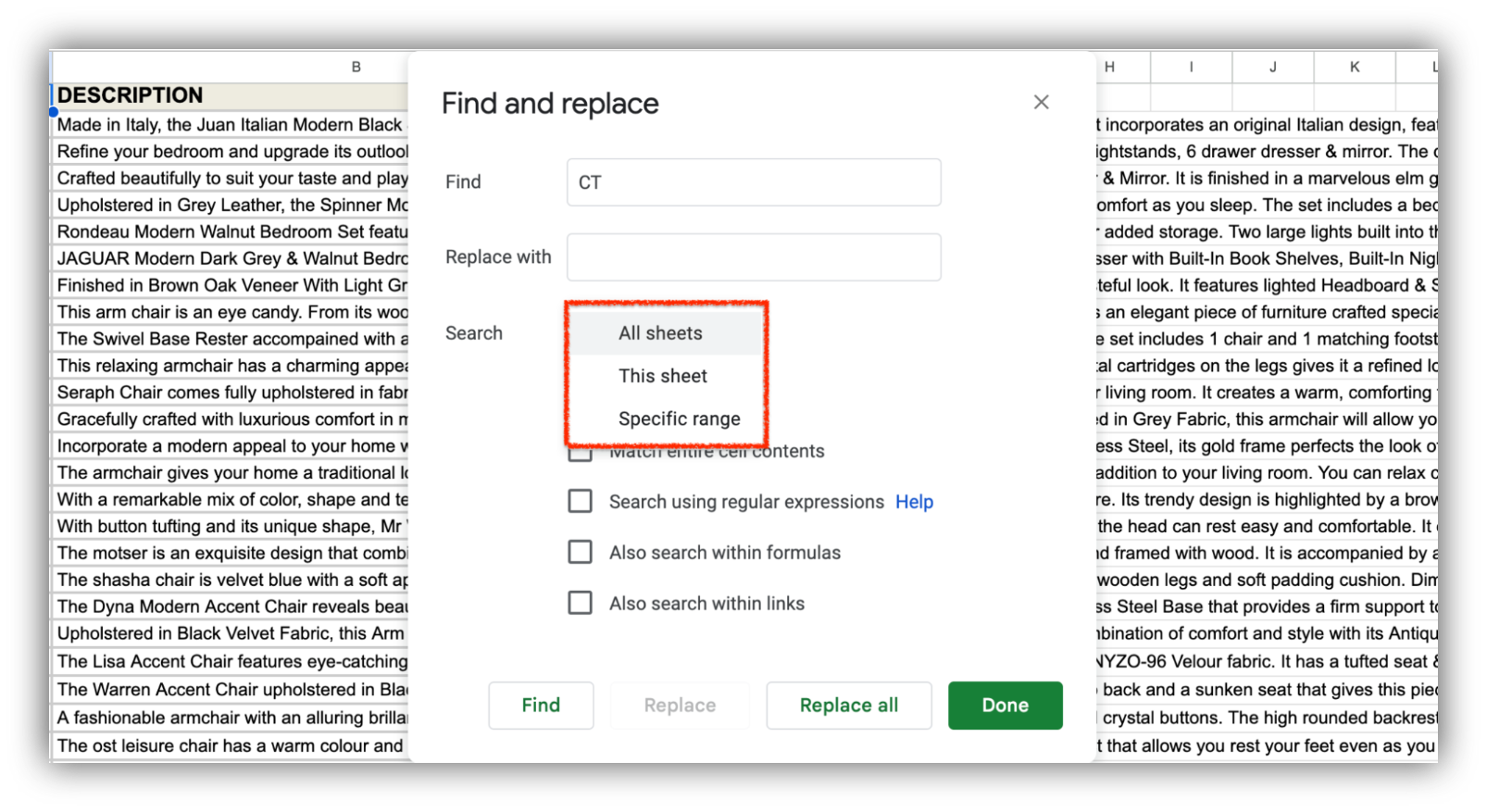
You have three options to choose from:

• Search all sheets: Google Sheets will scan through every sheet, including hidden sheets, and identify instances of your search term.
• Search this sheet: Google Sheets will restrict the search to the active sheet that you're working on to find instances of the search term within that specific sheet.
• Search specific range: Google Sheets will narrow down your search to a specific range within the active sheet to find what you’re looking for.

Step 4: (Optional) Customize your search using filters

To further modify your search, select any of the five options available:

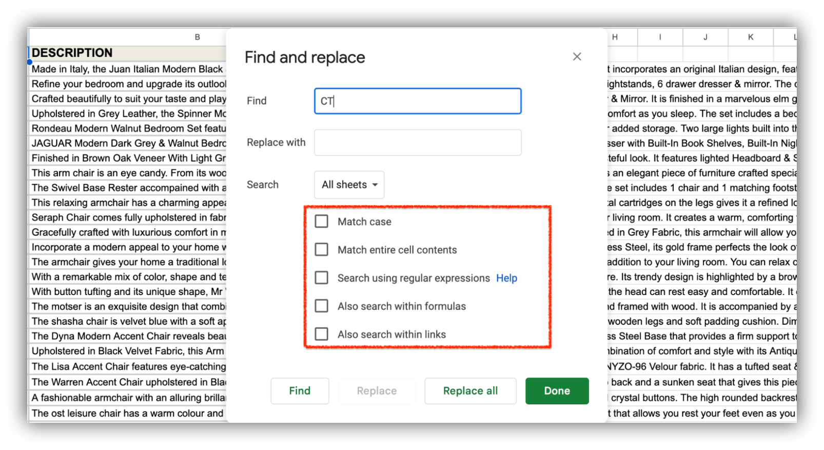
You can:

• Match case: ensures your search is case-sensitive, so only instances of the search term with the exact same letter case are considered matches
• March entire cell contents: finds cells with the exact search term. If you search for "apple," only cells with "apple" without any additional text will match
• Search using regular expressions: finds content with specific patterns, such as dates, phone numbers, or email addresses.
• Also, search within formulas: finds instances of the search term used in calculations or functions
• Also, search within links: includes cells with URLs that match the search term.

Step 5: Click the "Find" button to find instances

After completing the previous steps, click the "Find" button. This triggers Google Sheets to search for term instances within the current sheet or range.

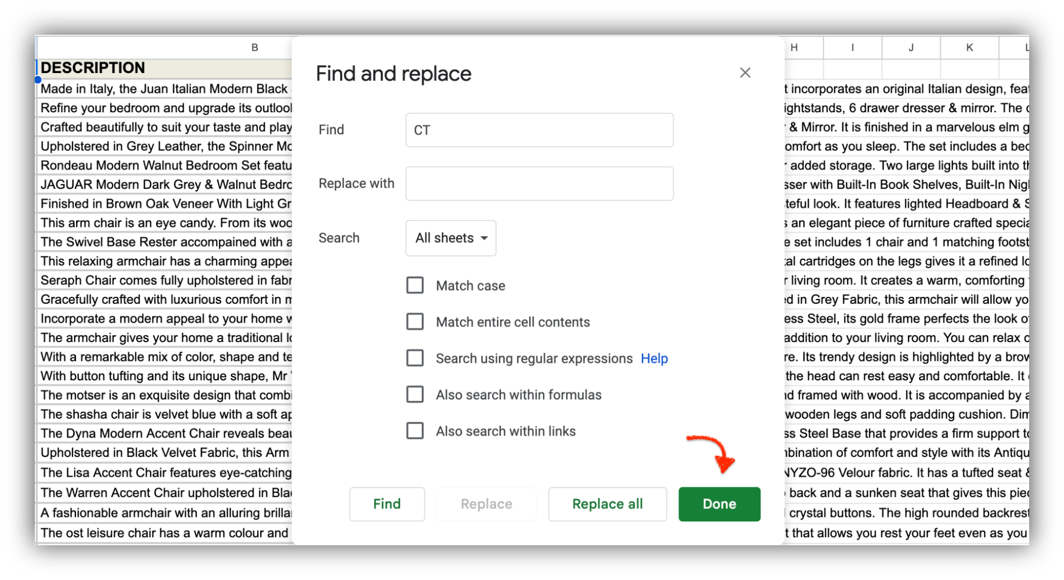
Step 6: Click "Done" when you've completed the task

Once you've completed your search (and any necessary replacements, if that was your intention), click Done to finish the search.

How to build a real search interface for Google Sheets with Softr

Cost: $0

Time: 3 minutes

The methods above all search the spreadsheet itself. That works when one person is hunting for a value, but it falls apart the moment a team shares the file. In a spreadsheet, filters, sorting, and hidden columns are global, so when one person filters to find a record, everyone else sees that same filtered view and people end up overwriting each other's work.

"In a spreadsheet, filters, sorting, and hidden columns are global, so users constantly overwrite each other's views. A database-driven app separates the interface from the underlying data, giving each user independent filters and role-specific landing pages with no collisions."

Softr fixes this by putting a real app on top of your data. It's a full-stack platform: an interface builder for the front end, native Softr Databases to store and structure your data, and Softr Workflows to automate the logic. You get a proper search bar, per-user filters, list and table views, and control over who sees what, all without writing code.

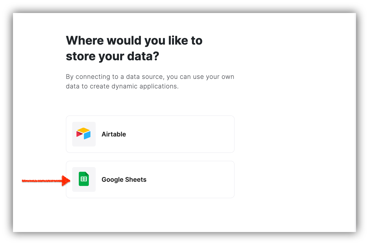
When it comes to where your data lives, you have options. You can use Softr Databases, or connect to Airtable, Google Sheets, and 17+ other data sources, including a REST API connector. For this tutorial we'll keep your existing Google Sheet as the data source and build a searchable interface on top of it.

The fastest way to get started is to describe what you need to the AI Co-Builder and let it generate a complete app for you. If you prefer, you can start from a template or build from a blank canvas instead. Here's how to set up search with Softr step by step.

Step 1: Log in to Softr or create an account

First, log in to your Softr account. If you don’t have an account, sign up for free.

Step 2: Connect your Google Sheets account to Softr

To start with Google Sheets, you need to go to your Application Settings and navigate to Data Sources. Next, click Connect a Data Source and select Google Sheets from the list.

You’ll have to log into the Google Account you want to connect to or select it if you’re already logged in.

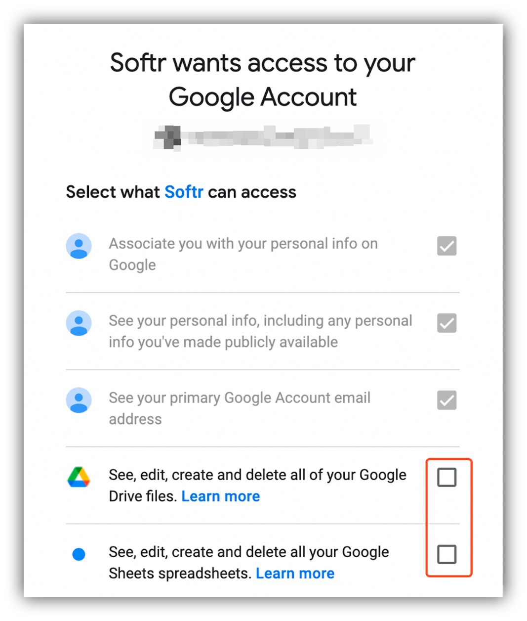
Then you need to authorize Softr to make changes in your associated account’s Google Sheets and Google Drive files. So, make sure to check the checkboxes highlighted below. Click Continue as soon as you’re done.

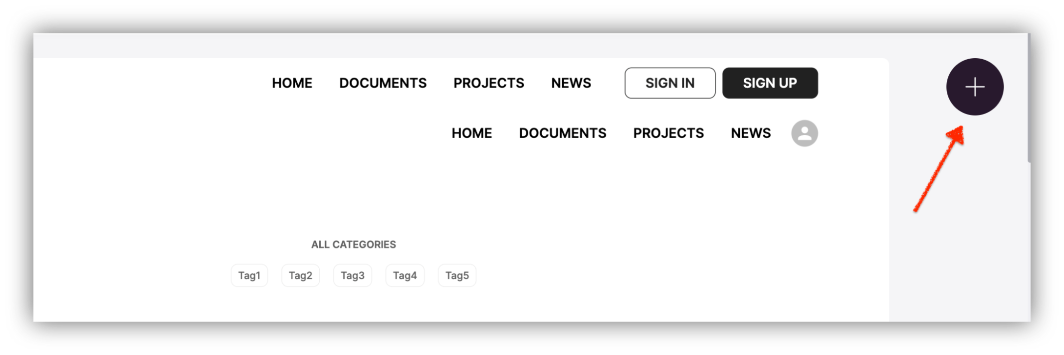
Step 3: Click the “+” sign to start selecting the Google Sheets you want to work on

After clicking the “+,” you'll find a sidebar with various blocks and components.

Browse through the dynamic blocks to find the ones that work with a data source, such as the List block, and choose any of the sheets from your library. Then select your connected Google Sheets account. You can also ask the AI Co-Builder to add the block and wire it to your data by describing what you need.

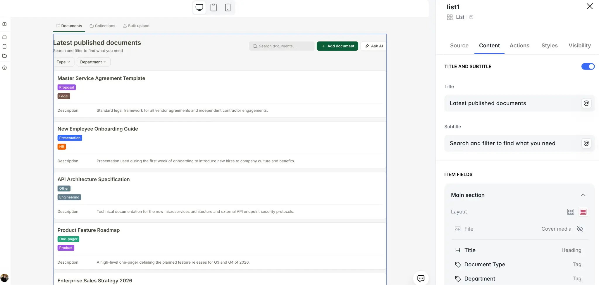
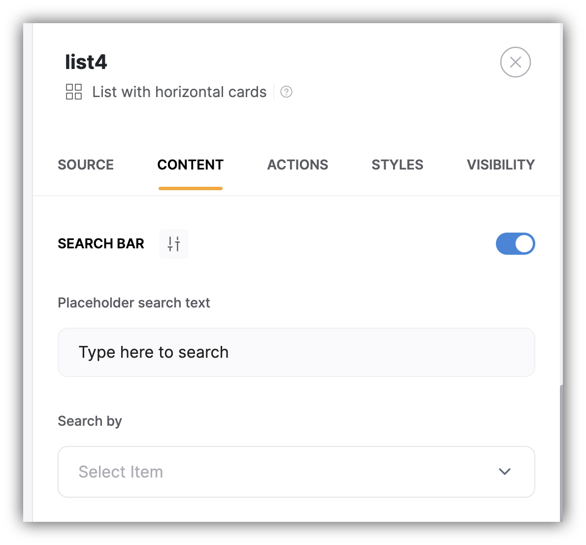
Step 4: Click the Content tab to set up the search bar

You can choose how you want your search bar to appear.

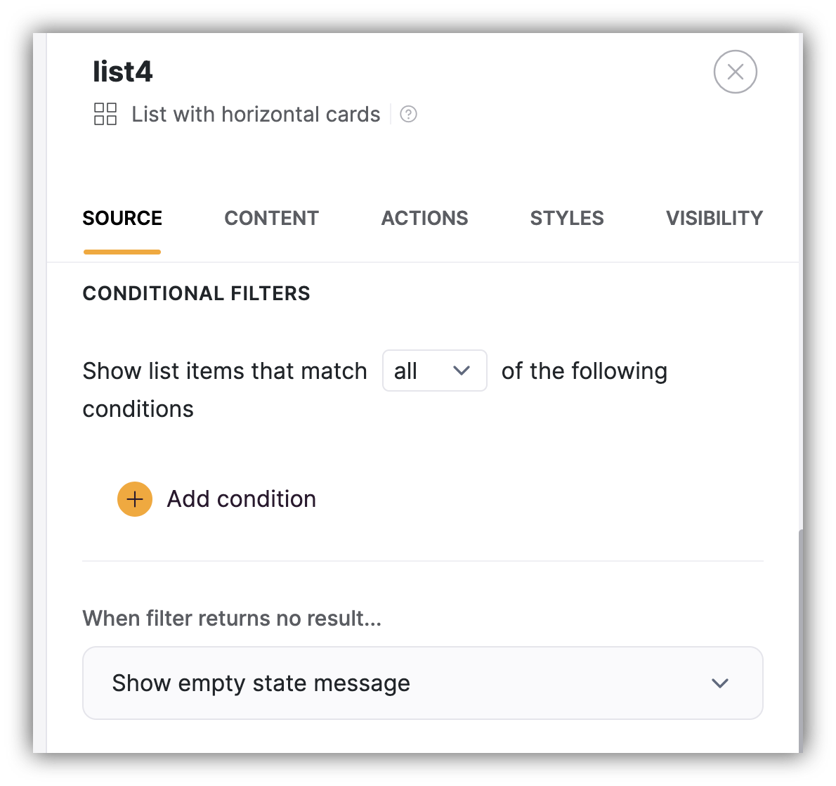
Step 5: Choose filters to find relevant results

Select search filters to get the most relevant results while searching.

Step 6: Test and optimize the search function

Click the “preview” button to test and ensure the search function works well.

How to search in Google Sheets using shortcuts

Cost: $0

Time: 30 seconds

Using keyboard shortcuts is one of the quickest ways to search in Google Sheets. Here’s a step-by-step breakdown to help you get started:

Step 1: Open your Google Sheets document

Open the Google Sheets document where you want to perform the search.

Step 2: Press "Ctrl + F" (Windows/ChromeOS) or "Cmd + F" (Mac) on your keyboard

To begin the search, press Ctrl (or Cmd on Mac) + F. This keyboard shortcut opens the "Find" dialog.

Step 3: Enter the text or value you want to search

In the "Find" dialog, type the word or phrase you want to search for. Google Sheets will automatically start highlighting instances of the search term as you type.

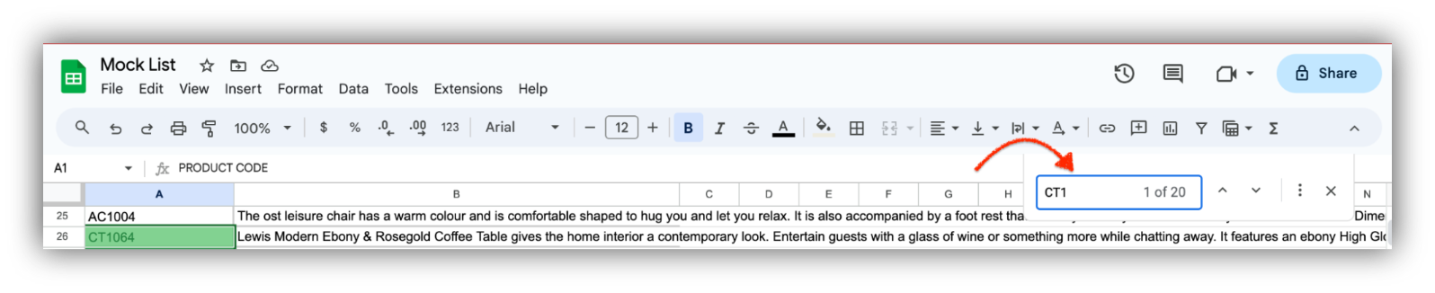
Step 4: Use the navigation arrows to move between instances

After inputting the search term, press Enter to find the first instance of the search term within the sheet. To find the next instance, use the arrows beside the search box.

Step 5: Click the "X" button or press the "Esc" key to close the box

To exit the "Find" dialog, press Esc or click the "X" button in the corner of the dialog.

How to search in Google Sheets using conditional formatting

Cost: $0

Time: 4 minutes

Conditional formatting allows you to visually highlight and format cells based on specific conditions. While it doesn't provide a direct way to search for data like functions do, you can use it to highlight data that matches certain criteria.

Here's how to use conditional formatting to achieve a search-like effect:

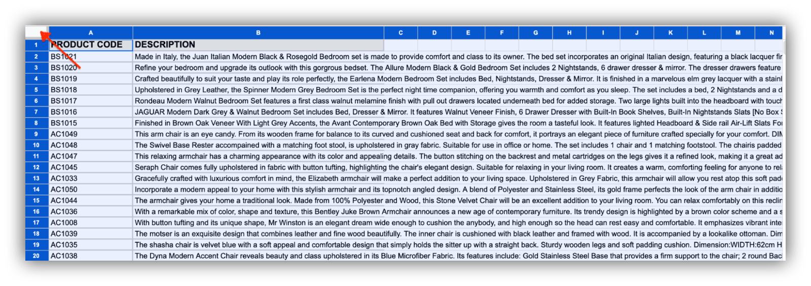
Step 1: Click and drag to select the range of cells you want to search

After opening the Google Sheet document, you want to work on, select the range of cells where you want to apply conditional formatting. There are two ways to do this.

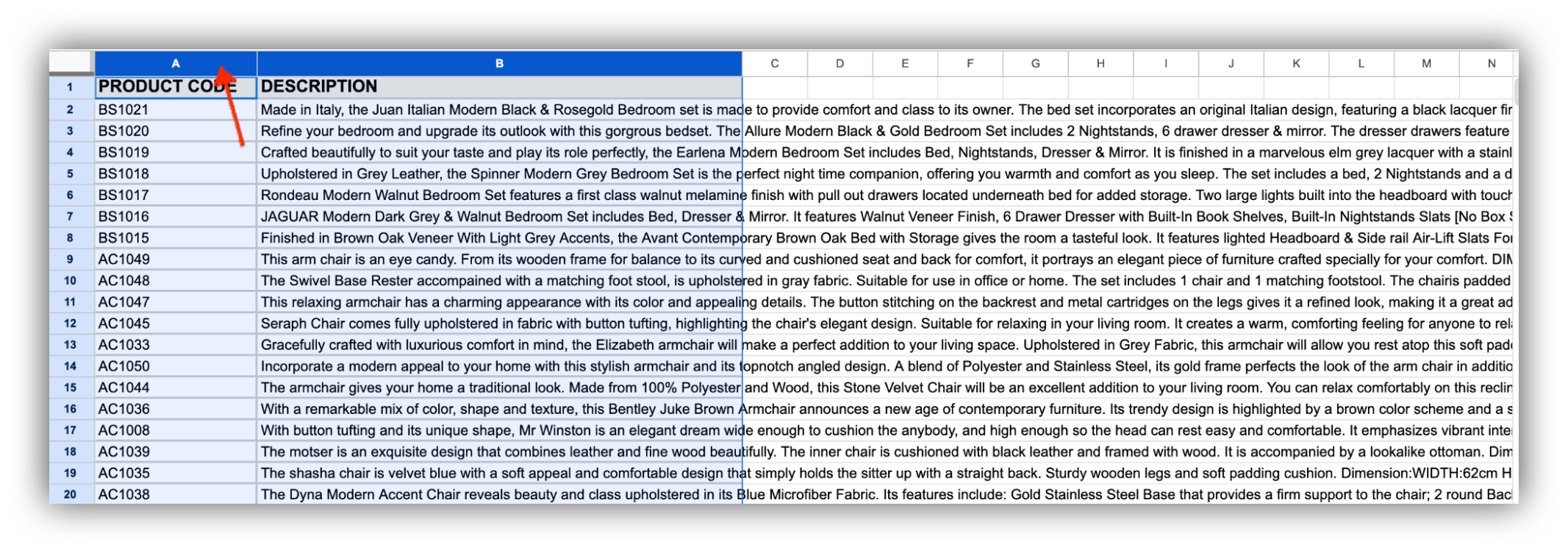
Click the area in the upper-left corner of the spreadsheet to select the entire sheet

Or click a column and drag to select the range of cells you want to search, depending on your needs.

Step 2: Click on Format > Conditional formatting from the menu

At the top of the Google Sheets interface, locate the menu bar and click on Format. From the dropdown menu, select Conditional formatting.

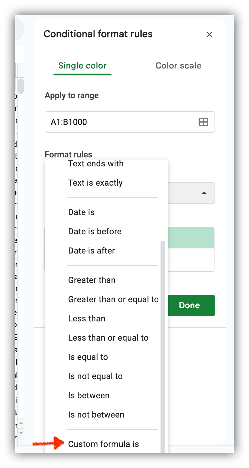
Step 3: Enter the formula that will match your search criteria

In the "Conditional format rules" sidebar that appears on the right, select the dropdown under "Format cells if" and choose "Custom formula is” from the list of options.

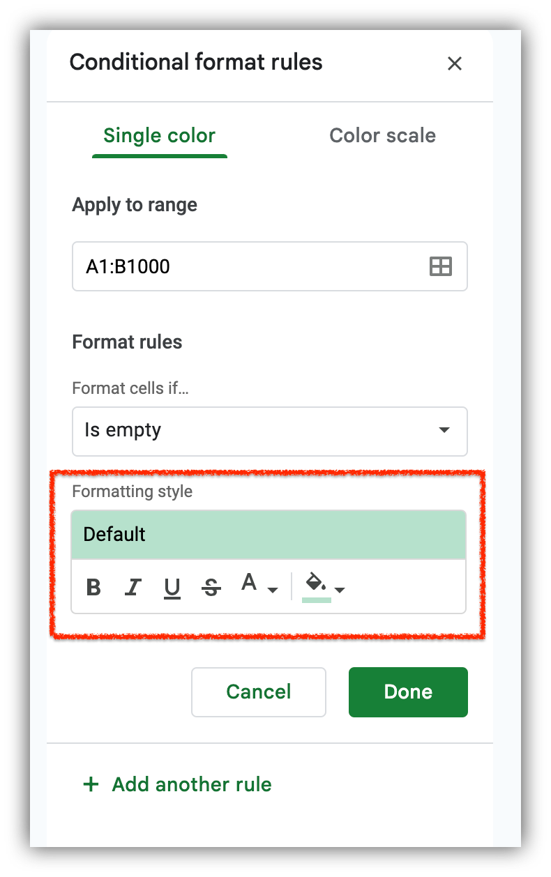
Step 4: Choose the formatting style you want for the selected range

Below the formula input, you can set the formatting style that you want to apply to cells that meet the condition. Click on the "Formatting style" dropdown to choose a style, such as text color, background color, or font style.

Step 5: Click "Done" to apply changes

Once you’re satisfied, click the "Done" button to apply the formatting.

How to search in Google Sheets using filter views

Cost: $0

Time: 3 minutes

Using Filter Views in Google Sheets allows you to create custom filtered versions of your data without affecting the view for others. It's a powerful way to focus on specific information. Here's how to use Filter Views to search in Google Sheets:

Step 1: Click on Data > Filter views > Create a new filter view

Click and drag to select the range of cells containing the data you want to search through. In the menu bar at the top, click on Data and select Filter views from the dropdown menu, then choose Create a new filter view.

Step 2: Set conditions for each column using the filter options

A filter panel will appear at the top of your sheet, like the one highlighted in the screenshot below.

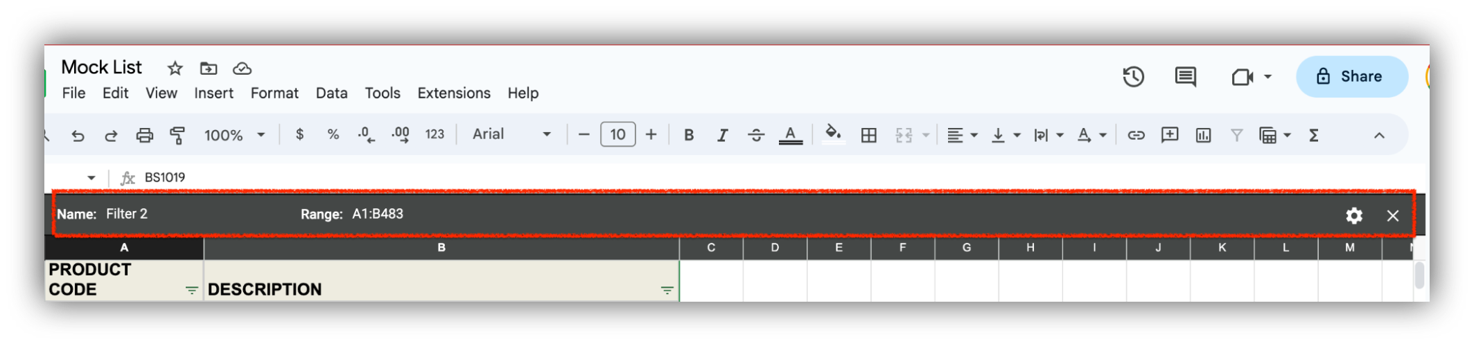
In the first row of the filter panel, you'll see dropdowns for each column header in your selected range.

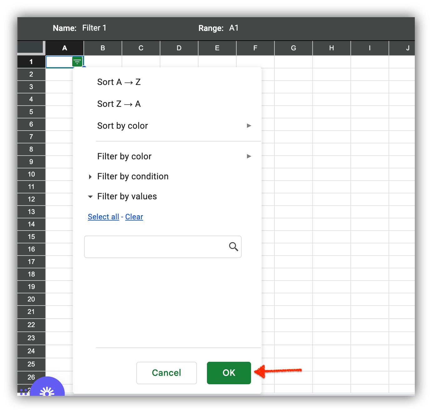
Step 3: Click on the column dropdown where you want to apply a filter

In the filter view toolbar that appears at the top of the sheet, click on the filter icon (funnel-shaped icon) next to the header of the column you want to search. This will open the filter options for that column.

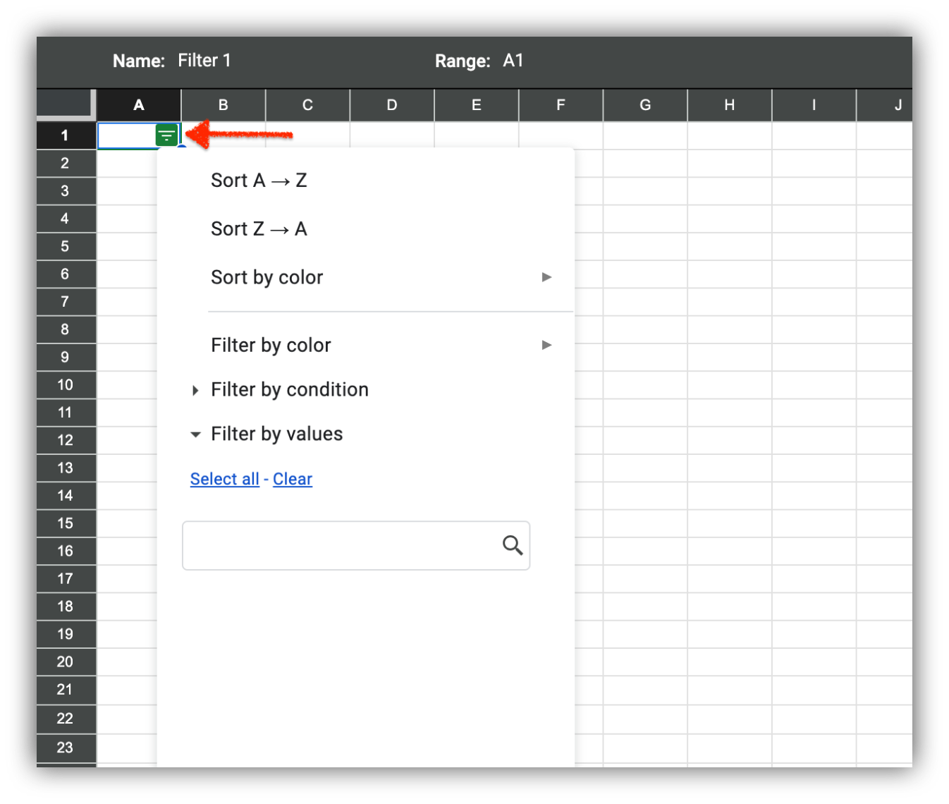
Depending on the data type in the column, you can select various filter criteria such as text, numbers, colors, dates, and more. You can also apply multiple filters by choosing another column's filter and criteria. Google Sheets will combine the filters to show rows that meet all the selected criteria.

Step 4: Click Save to create the filter view

After selecting the filter criteria, click "OK" or press Enter. The filter view will be applied, showing only the rows that match the selected criteria.

You'll notice that only the rows that meet your filter criteria are visible, while the rest of the data is temporarily hidden.

How to search Google Sheets using VLOOKUP Function

Cost: $0

Time: < 1 minute

VLOOKUP is great for fast searches and simple data retrieval. Yet, it has restrictions: you can only search the first column of a table and sort data for close matches.

Step 1: Identify the search criteria

Determine the value you want to search for. This could be a specific name, ID, or any other unique identifier. For example, if you have a table of products in columns A, B, and C, you could make finding the price of "Product B" your priority.

Step 2: Choose a cell for the VLOOKUP result

Decide on a cell where you want the result of the VLOOKUP function to appear.

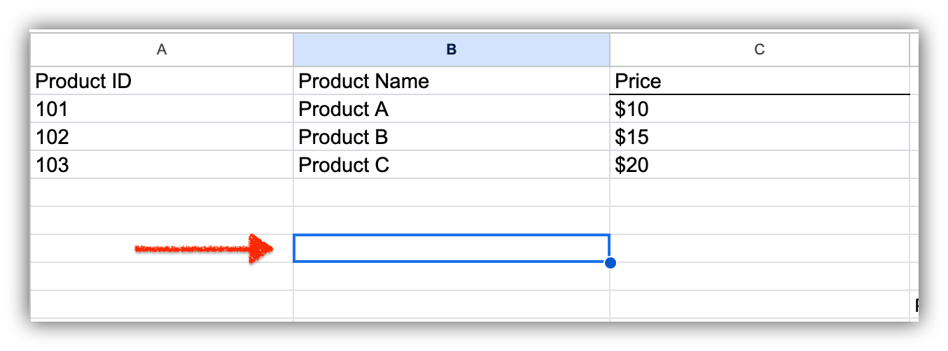
This cell will display the result based on your search.

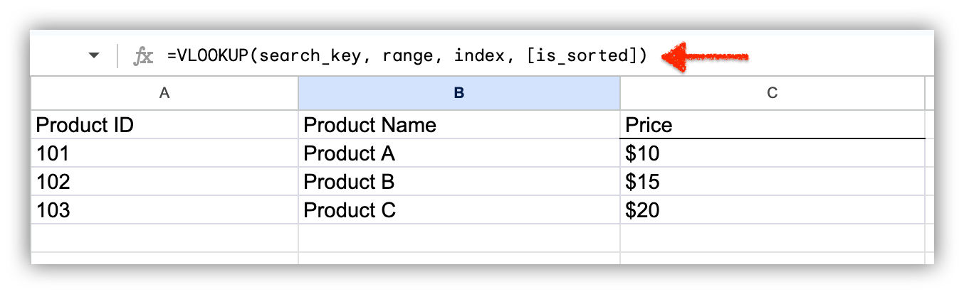
Step 3: Set up the VLOOKUP function

In the cell where you want the result, type the following formula: =VLOOKUP(search_key, range, index, [is_sorted])

Step 4: Fill in the parameters

To do this, you should be clear on what you’re replacing each parameter with:

• search_value: Replace this with the value you're searching for (e.g., the name or ID you identified earlier).
• range: Specify the range where the data is located. This should include the column with the search criteria and the column with the corresponding information you want to retrieve.
• index: Indicate the column number (starting from 1) that contains the information you want to retrieve based on the search.
• is_sorted: Enter TRUE if your data is sorted in ascending order or FALSE if it's not sorted.

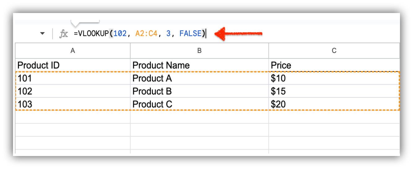
Here, 102 is the lookup value, A2:C4 is the table range, 3 indicates the third column (which is the price column), and FALSE specifies an exact match.

Step 5: Hit “Enter” to get the search result

After filling in the parameters, press Enter, and the VLOOKUP function will retrieve the desired information based on the search criteria you provided.

The result in this case is “Product B.”

How to search Google Sheets using HLOOKUP Function

Cost: $0

Time: < 1 minute

The HLOOKUP function allows you to search for a value in the first row of a range and retrieve a corresponding value from another row within the same column.

Step 1: Identify the search criteria

Determine the value you want to search for horizontally. This could be a specific name, ID, or any other unique identifier. For example, if you have a table of products in columns A, B, and C, you could make finding the price of "Product A" your priority.

Step 2: Choose a Cell for the HLOOKUP Result

Select a cell where you want the result of the HLOOKUP function to appear. This cell will display the information retrieved based on your search.

Step 3: Set Up the HLOOKUP Function

To search using this function, use the formula “=HLOOKUP(search_key, range, index, [is_sorted]).”

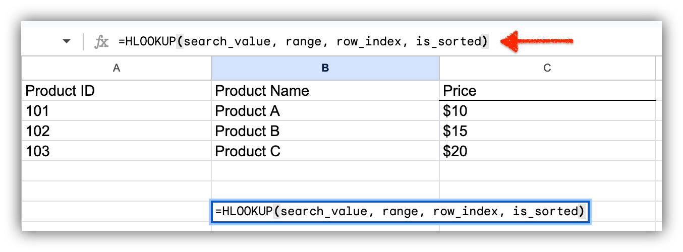
Step 4: Fill in the parameters

To do this, you should be clear on what you’re replacing each parameter with:

• search_key: Replace this with the value you're searching for horizontally (e.g., the name or ID you identified earlier).
• range: Specify the range where the data is located. This should include the row with the search criteria and the rows with the corresponding information you want to retrieve.
• row_index: Indicate the row number (starting from 1) that contains the information you want to retrieve based on the search.
• is_sorted: Enter TRUE if your data is sorted in ascending order or FALSE if it's not sorted.

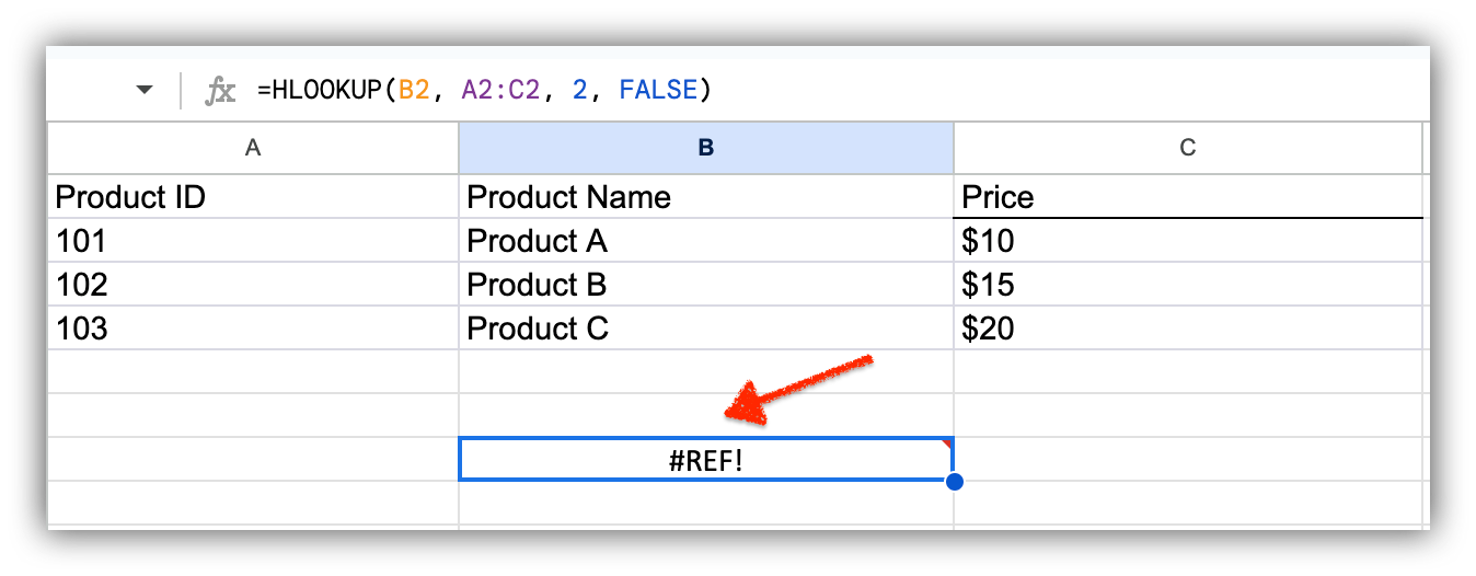
After filling in the parameters, press Enter, and the HLOOKUP function will retrieve the desired information based on the search criteria you provided.

HLOOKUP is limited to searching the first row of the range for values, so if the search value is not found, it may return an error or an undesired result.

How to search using INDEX and MATCH functions

Cost: $0

Time: < 1 minute

The combination of the INDEX and MATCH functions in Google Sheets is a powerful way to perform more flexible and dynamic searches.

Using both functions together provides more flexibility than VLOOKUP or HLOOKUP, as you can search based on various criteria and retrieve data from different rows and columns in your sheet.

Step 1: Choose your search criteria and the cell to display the result

Identify the value you want to search for and select the cell (or cells) where you want the result of the INDEX and MATCH functions to appear.

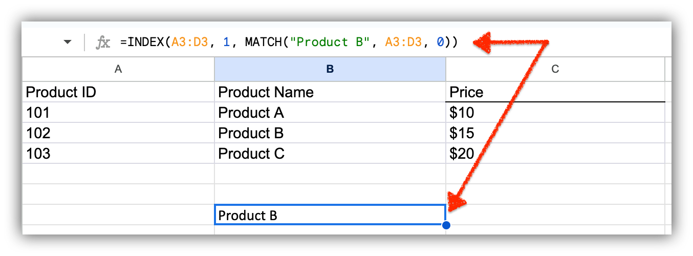
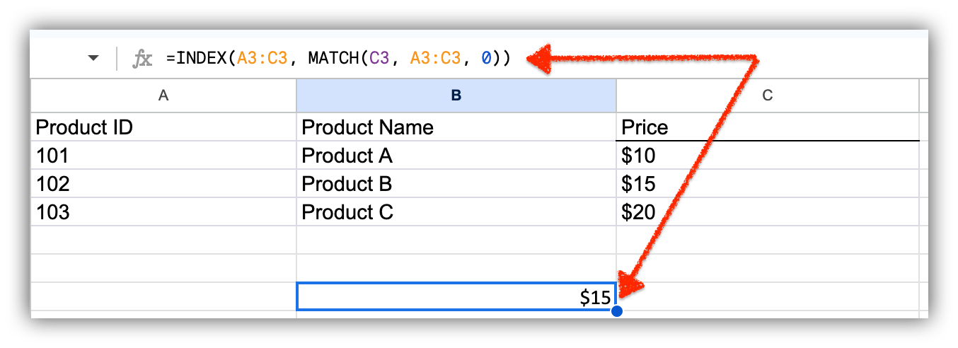
Step 2: Set up the INDEX and MATCH functions

Suppose you want to find the price of "Product B" using the INDEX and MATCH functions. In the cell where you want the result, type the following formula: =INDEX(range_to_return, MATCH(search_value, search_range, 0))

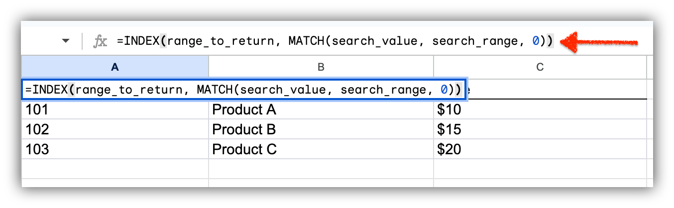
Step 3: Fill in the parameters

For the parameters,

• range_to_return: Specify the range that contains the information you want to retrieve based on the search. This range should include the data you want to display when a match is found.
• search_value: Replace this with the value you're searching for (e.g., the name or ID you identified earlier).
• search_range: Specify the range where the search value should be located. This range should include the column or row containing the search criteria.

After entering the formula, press Enter. The INDEX and MATCH functions will work together to retrieve the desired information based on the search criteria you provided.

Step 4: Review the Result

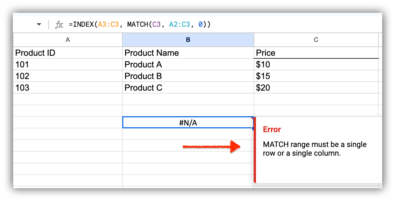
The cell where you entered the formula will display the result of the INDEX and MATCH functions. If the search value is found in the specified search range, it will show the corresponding information. If it isn't, it might display an error message.

How to search using QUERY Function

Cost: $0

Time: < 1 minute

The QUERY function in Google Sheets allows you to perform SQL-like queries on your data. It is incredibly flexible and can handle more complex queries involving sorting, grouping, and filtering. This is especially useful when handling larger datasets or when you need to combine and manipulate data from multiple sheets.

If you're familiar with SQL, you can use this function to perform advanced searches.

Step 1: Identify the search criteria

Determine the conditions you want to use for your search. This could involve specifying columns, conditions, sorting, and more.

Step 2: Choose a cell for the Query result

Select a cell or range of cells where you want the result of the QUERY function to appear. This is where the retrieved data based on your search will be displayed.

Step 3: Set Up the QUERY Function

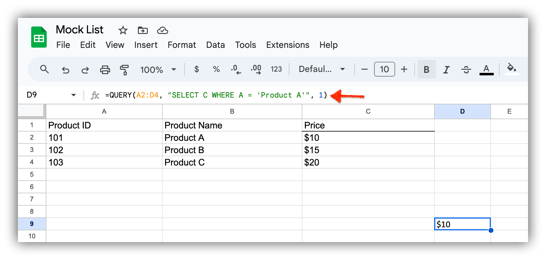
In the cell where you want the result, type the following formula: =QUERY(data_range, query_expression, headers), where:

• data_range: The range of data you want to query, including headers.
• query_expression: Your SQL-like query expression is enclosed in double quotes.
• headers: A number (1 or 0) indicating whether your data range has headers.

For example, using the same table, you can retrieve the price of "Product A" with the same expression. The formula will return the price of $10 in the cell where you placed it.

Step 4: Review the Result

The cell where you entered the formula will display the result of the QUERY function. If the data matches your query expression, it will show the retrieved rows. If the syntax is off or nothing matches, it might display an error message instead.

When to stop searching the sheet and build an app

The nine methods above all share one limit: they search the spreadsheet, and the spreadsheet stays the place everyone works. That's fine for personal use. Lookup functions can break too, since VLOOKUP and INDEX/MATCH match text strings, so renaming a value like a company name can quietly break every formula that referenced it. A relational database avoids that by linking records through unique identities instead of text.

A simple heuristic helps here: if a spreadsheet is the weekly operational backbone for two or more people, it's worth turning into an app. Below that threshold, the coordination costs usually stay manageable. Above it, people waste time scrolling, filters collide, and there's no real control over who sees what.

"I find Softr to be the easiest system to connect a database to. As someone less technical, I find it helpful that working with a database in Softr is similar to an Excel spreadsheet. The initial setup was very easy for me since I used the AI assistant, which I thought was very in tune with what I was looking for." - Joe L., Sales and Strategic Partnerships, G2 review

With Softr, you can turn your Google Sheets data into a custom business app, such as a portal, CRM, tracker, or dashboard, complete with a search bar and per-user filters. Users and permissions let you control exactly what each person can view and edit, so everyone finds the records they need without scrolling through a shared sheet. The quickest path is to describe your tool to the AI Co-Builder and let it generate the app, then refine it from there.

Ready to go further than search? Build a user interface for your Google Sheets data and give your team a single place to find, view, and update records.